Create Execution-Time Profile for Deployed ROS 2 Nodes Using XCP-Based External Mode
R2026bThis topic shows how to measure execution time of a ROS 2 node generated in Simulink® and running in XCP-based external mode. The example also shows how to analyze
the results using the Code Profile
Analyzer (Embedded Coder) (Simulink
Coder™) and Simulation Data
Inspector (Simulink) (Simulink) (SDI) apps. You can also analyze the measurements within the MATLAB® environment using a workspace variable of type
coder.profile.ExecutionTime.
In a Simulink model, the sample times you specify determine the time schedule for running generated code on target hardware. With enough computing power on the hardware, the code runs in real time according to the specified sample times. Code execution profiling enables you to check whether the generated code for your deployed ROS 2 node meets your real-time performance requirements.
When you deploy the node using XCP-based external mode, Simulink Coder automatically instruments the generated code with timing hooks. The instrumented code then streams wall-clock execution-time metrics for tasks and functions via XCP back to Simulink for analysis.
You can use these profiling results to improve your system design. For example, you can:
Identify bottlenecks by pinpointing the tasks and functions that consume the most execution time.
Optimize expensive components by trading functionality for speed where real-time requirements are not met.
Note
Code execution profiling requires XCP on TCP/IP as the communication interface. Code execution profiling is not available with the TCP/IP communication interface. Profiling supports applications running on both a local host machine and a Linux remote machine. The system target file must be ERT or ERT based.
Code Execution Profiling Parameters
To configure code execution profiling, open the model configuration parameters dialog box. Navigate to Code Generation > Verification and enable the Measure task execution time parameter under Code execution time profiling.
Measure Function Execution Time
(CodeExecutionProfiling)
This parameter controls the granularity of code instrumentation beyond task-level profiling. Select one of the following options:
| Profiling Option | Description | When to Use |
|---|---|---|
Off | Simulink
Coder instruments only at the task level (in
| To identify the most time-consuming tasks without drilling into individual function calls. This option is the least intrusive and has the smallest performance overhead. |
Coarse (referenced models and subsystems
only) | Simulink
Coder instruments at the task level and also around
calls to referenced models and atomic subsystem functions (in
| To see execution time for referenced models and subsystem boundaries without timing every individual function call. This option provides a balance between detail and overhead. |
Detailed (all function call
sites) | Simulink
Coder instruments at the task level and around all
function calls in the model code (in
| To pinpoint exactly which function is a bottleneck with the finest granularity. This option has the highest performance overhead due to the large number of instrumentation points. |
Tip
For function-level instrumentation to take effect in a referenced model, you must enable Measure task execution time in the top model. Then, for each Model block you want to profile, enable Measure function execution times only at the specific reference level where you need those measurements.
Specify Workspace Variable
(CodeExecutionProfileVariable)
Specify the name of a MATLAB workspace variable that holds execution-time measurements after the
profiling session ends. The default variable name is
executionProfile. When the simulation ends, the software
generates a variable with this name in the MATLAB base workspace. The variable contains the execution-time measurements
and is a class of type coder.profile.ExecutionTime.
Save Profiling Data
This parameter controls how much profiling data the software saves to the workspace and whether it streams execution times to SDI during the simulation.
This table explains the differences between the save options:
| Feature | Summary data only | All data | Metrics only |
|---|---|---|---|
| Real-time data | Available | Available | Not available. Target sends profiling data only at the end of the simulation. |
| Host memory requirement | Requires less memory as the host stores only summary metrics of profiling data | Requires large memory as the host stores all the data sent by the target | Requires less memory as the host stores only the metrics data sent by the target |
| SDI streaming | Available | Available | Not available |
| Bandwidth requirement | Requires additional bandwidth | Requires additional bandwidth | Does not require additional bandwidth |
Use the following information to select the recommended save options in different scenarios:
Summary data only — Select this option if the simulation is running for a long time and the host does not have a lot of memory. You can still generate a report and stream execution times to the SDI during the simulation.
All data — Select this option if the host has enough memory and the target has the required bandwidth to stream data. After the simulation, you can use methods from the
coder.profile.ExecutionTimeclass to retrieve execution-time measurements for every call to each profiled section of code.Metrics only — Select this option if the target does not have enough time or bandwidth to stream profiling data. On the target hardware, the software stores maximum execution times, average execution times, and number of calls. At the end of the simulation, Simulink uploads this summary data from the target hardware to your development computer.
Profile Execution Time of ROS 2 Node on Local Host
This example shows how to measure execution time of a ROS 2 node generated in Simulink® and running in XCP-based external mode. The example also shows how to analyze the results using the Code Profile Analyzer (Embedded Coder) and Simulation Data Inspector (Simulink) (SDI) apps.
Prerequisites
Before you begin, ensure you have:
A Simulink model configured for ROS 2 code generation.
XCP on TCP/IP selected as the communication interface for external mode. For details on configuring external mode, see the Feedback Control of ROS 2 Robot with XCP-Based External Mode example.
Enable Code Execution Profiling
1. Open the Simulink model configured for ROS 2 code generation. In the Prepare section on the ROS tab, click Hardware Settings to open the Configuration Parameters dialog box.
open_system("proportionalControllerCodeProfiling.slx")![Simulink model titled "Proportional Controller with XCP on TCP/IP External Mode" showing a Proportional Controller subsystem with four constant inputs (Desired position [10 10], Position X, Position Y, and Orientation theta) and two outputs (Linear Velocity and Angular Velocity) connected to publish blocks.](../../examples/ros/ProfileExecutionTimeOfROS2NodeOnLocalHostExample_01.png)
2. In the Configuration Parameters dialog box, navigate to Code Generation > Verification. Under Code execution time profiling, select the Measure task execution time parameter to enable task-level execution-time measurement.
3. Set the Measure function execution times parameter to Detailed (all function call sites) to measure execution time for all function calls in the generated code.
4. To configure how profiling results are stored:
In the Workspace variable field, specify a variable name (for example,
executionProfile) to store execution-time measurements.Set Save options to
Summary data onlyto stream to SDI and store minimal end-of-run data.
5. Click OK to apply the configuration.
Run XCP-Based External Mode Session
On the ROS tab, in the Connect section, verify that the Deploy To option is set to
Localhost.On the Run On Hardware tab, select Monitor & Tune. Simulink builds the instrumented code, deploys it, and starts the XCP-based external mode session. Because you selected
Summary data onlyas the save option, execution-time data begins streaming to SDI.Let the simulation run long enough for execution-time measurements to stabilize.
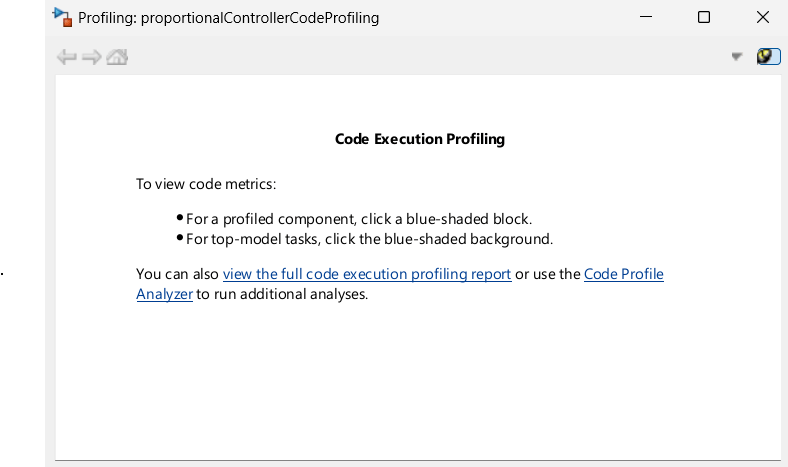
Click Stop on the Hardware tab to end the profiling session. The Code Execution Profiling dialog box that opens includes direct links to open the generated report and Code Profile Analyzer app.
Analyze Results Using Code Profile Analyzer
When the profiling session is complete, you can view execution-time metrics through a display panel, report, or in the Code view using the Code Profile Analyzer app.
1. After the simulation ends, the software stores execution-time profiling data in the workspace variable you specified (for example, executionProfile). The software also generates a profiling report with execution-time metrics for all profiled tasks and functions.
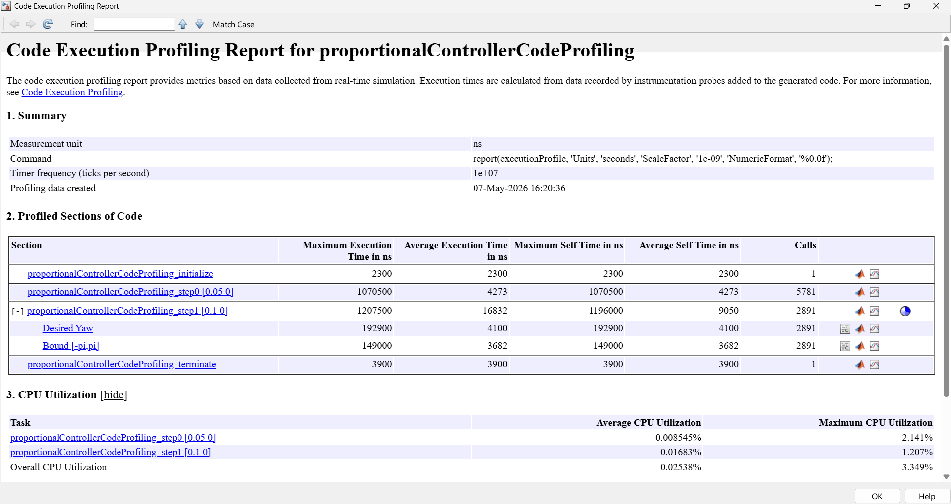
2. Open the Code Profile Analyzer app to examine task and function execution times. The analyzer provides a summary of:
Execution time per task and per function (if you enabled function-level instrumentation)
Maximum, average, and total execution times
Number of calls for each profiled section
![Code Profile Analyzer app showing the Function Execution tab. The left pane displays a model hierarchy tree with profiled sections. The center table lists section names and corresponding function names including initialize, step0, step1, Desired Yaw, Bound [-pi,pi], and terminate functions. The Relative Function Execution Times table below shows self time as a percentage of caller, task, and simulation for each section. The Summary pane on the right shows the profiled component, workflow (XCP External Mode), environment (Simulink), save options (Summary data only), and time created.](../../examples/ros/ProfileExecutionTimeOfROS2NodeOnLocalHostExample_04.png)
3. Generate a detailed execution-time report from the app for offline analysis.
You can also use the Code Profile Analyzer app to configure and validate execution-time profiling settings for a model hierarchy. On the General tab, click Configure Models to load a top model and control function profiling settings for referenced models. Click Validate Configuration to verify settings across the hierarchy before running the simulation.
Visualize Execution Metrics in Simulation Data Inspector (SDI)
You can use the Simulation Data Inspector (SDI) to view and compare the variation of execution times over a simulation.
Open the SDI by clicking the Data Inspector button under Review Results tab of the toolstrip.
In the Inspect pane, expand the profiling run to view execution-time signals. You can:
Compare execution-time trends across time steps to identify variability.
Overlay signals from multiple profiling runs to detect regressions.
Export data for further analysis.
![Simulation Data Inspector showing the Inspect pane with a Profiling node expanded to display execution-time signals for the proportionalControllerCodeProfiling model. Three signals are selected and plotted: initialize (blue), step0 [0.05 0] (orange), and step1 [0.1 0] (green). The time-series plot shows execution time in seconds on the y-axis and simulation time on the x-axis, with step1 exhibiting the highest variability and peak execution times around 0.0001 seconds.](../../examples/ros/ProfileExecutionTimeOfROS2NodeOnLocalHostExample_05.png)
See Also
Code Profile Analyzer (Embedded Coder) | Simulation Data Inspector (Simulink)

