GPS Waveform Generation
This example shows how to generate Global Positioning System (GPS) legacy navigation (LNAV) data, civil navigation (CNAV) data, and a complex baseband waveform. The spreading of the data is performed with coarse acquisition code (C/A-code), precision code (P-code), or civil moderate / civil long code (L2 CM-/L2 CL-code). This example shows GPS waveform generation according to the IS-GPS-200 standard [1]. To design a navigation system based on GPS, you must test the receiver with a received signal. Because you cannot control transmitter and channel parameters, a signal that is received from a satellite is not useful for testing a receiver. To test the receiver, you must use a waveform that is generated under a controlled set of parameters.
This example shows how to generate a GPS waveform for one satellite without any impairments. For a realistic GPS waveform generation from multiple satellites refer GNSS Signal Transmission Using Software-Defined Radio Example.
Introduction
Generate a GPS signal by using these three steps.
Generate GPS data bits by using the configuration parameters that are described in later sections. The data bits are generated at a rate of 50 bits per second (bps).
Spread these low rate data bits by using high rate spreading codes. The GPS standard IS-GPS_200 [1] specifies three kinds of spreading codes: C/A-code, P-code, and L2 CM-/L2 CL-code. In addition to these three codes, this standard also specifies Y-code to use instead of P-code when anti-spoofing mode of an operation is active. P-code and Y-code together are called P(Y)-code. The configuration parameters determine the spreading code that is used to generate the waveform.
Generate the GPS complex baseband waveform from the bits that are spread by the spreading codes by selecting codes on the in-phase branch and quadrature-phase branch according to the set of configuration parameters.
This figure shows the block diagram of the GPS waveform generator from the configuration parameters.

GPS Signal Structure
The standard [1] describes the transmission of GPS signals on two frequencies: L1 (1575.42 MHz) and L2 (1227.60 MHz). A signal of base frequency 10.23 MHz generates both of these signals. The carrier frequency of L1 is 154 x 10.23 MHz = 1575.42 MHz, and the carrier frequency of L2 is 120 x 10.23 MHz = 1227.60 MHz. This example demonstrates the generation of a GPS baseband signal. The generated waveform can be upconverted to either L1 or L2 frequencies, depending on your requirements. According to the standard, the legacy signal is transmitted on both L1 and L2 frequencies. Therefore, this example gives you the flexibility to generate either a legacy waveform or an L2C waveform in baseband, excluding the carrier frequency information. The relationship between the standard-specified signal structure and the MATLAB® baseband waveform generation options is illustrated in this figure.
To select the content for transmitting over the in-phase and quadrature-phase branches, use this table.
signalType ="legacy" % Possible values - "legacy" | "l2c"
signalType =
"legacy"
hasDataWithPCode =true; % When set to false, only spreading code is modulated without any data with it hasDataWithCACode =
true; % When set to false, only spreading code is modulated without any data with it
Set the showVisualizations property to enable the spectrum and correlation plot visualizations. Set the writeWaveformToFile property to write the complex baseband waveform to a file if needed. This example enables visualizations and disables writing the waveform to a file.
showVisualizations =true; writeWaveformToFile =
false;
Specify the satellite PRN index as an integer in the range [1,63].
PRNID = 1;
sampleRate = 4*10.23e6; % 4 time the rate of P-code to be able to see the side lobes of the spectrum
Because generating the GPS waveform for the entire navigation data can take a lot of time and memory, this example demonstrates generating a waveform for only one bit of the navigation data. You can control generating the waveform for a specified number of data bits by using the property NumNavDataBits.
% Set this value to 1 to generate the waveform from the first bit of the
% navigation data
NavDataBitStartIndex = 1321;

% Set this value to control the number of navigation data bits in the
% generated waveform
NumNavDataBits = 1;
GPS Data Initialization
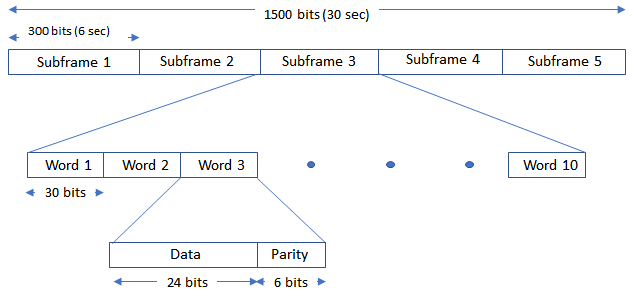
Many of the transmitted properties in the LNAV and CNAV data are same, but the frame structure is different. The LNAV data is transmitted in 1500 bit-length frames, with each frame consisting of five subframes of 300 bits in each subframe. Because the data rate is 50 bps, transmitting each subframe takes 6 seconds and transmitting each frame takes 30 seconds. Each subframe consists of 10 words with 30 bits (24 data bits and 6 parity bits) in each word. The GPS data contains information regarding the clock and the position of the satellites. This figure shows the frame structure of the LNAV data.
The CNAV data is transmitted continuously in the form of message types. Each message type consists of 300 bits that are transmitted at 25 bps. These bits are passed through a rate-half convolutional-encoder to obtain 600 bits from each message type at 50 bps. Transmitting each message type takes 12 seconds. The standard [1] defines 14 message types in this order: 10, 11, 30, 31, 32, 33, 34, 35, 36, 37, 12, 13, 14, and 15. For a detailed description of each message type and the data transmitted, see IS-GPS-200L Appendix III [1]. The order in which each message type is transmitted is completely arbitrary but is sequenced to provide optimal user experience. In this example, you can choose the order in which these message types are transmitted. This figure shows the CNAV message structure.
The message type shown in this figure has these fields:
PRN ID: Pseudo-random noise (PRN) index
MSG: Message
TOW: Time of week
CRC: Cyclic redundancy check
Initialize the data configuration object to generate the CNAV data. You can create a configuration object from the HelperGPSNavigationConfig object. Update the configuration object properties to customize the waveform as required.
cnavConfig = HelperGPSNavigationConfig(SignalType = "CNAV", PRNID = PRNID)cnavConfig =
HelperGPSNavigationConfig with properties:
SignalType: "CNAV"
PRNID: 1
MessageTypes: [4×15 double]
HOWTOW: 1
L2CPhasing: 0
SignalHealth: [3×1 double]
WeekNumber: 2149
GroupDelayDifferential: 0
ReferenceTimeOfClock: 0
SemiMajorAxisLength: 26560000
ChangeRateInSemiMajorAxis: 0
MeanMotionDifference: 0
RateOfMeanMotionDifference: 0
Eccentricity: 0.0200
MeanAnomaly: 0
ReferenceTimeOfEphemeris: 0
HarmonicCorrectionTerms: [6×1 double]
IntegrityStatusFlag: 0
ArgumentOfPerigee: -0.5200
RateOfRightAscension: 0
LongitudeOfAscendingNode: -0.8400
Inclination: 0.3000
InclinationRate: 0
URAEDID: 0
InterSignalCorrection: [4×1 double]
ReferenceTimeCEIPropagation: 0
ReferenceWeekNumberCEIPropagation: 101
URANEDID: [3×1 double]
AlertFlag: 0
AgeOfDataOffset: 0
AlmanacFileName: "gpsAlmanac.txt"
Ionosphere: [1×1 struct]
EarthOrientation: [1×1 struct]
UTC: [1×1 struct]
DifferentialCorrection: [1×1 struct]
TimeOffset: [1×1 struct]
ReducedAlmanac: [1×1 struct]
TextInMessageType36: 'This content is part of Satellite Communications Toolbox. '
TextInMessageType15: 'This content is part of Satellite Communications Toolbox. '
In theory, clocks of all satellites must be synchronized, which implies that all GPS satellite clocks must show the same time at a given moment in time. In practice, deterministic satellite clock error characteristics of bias, drift, and aging as well as satellite implementation characteristics of group delay bias and mean differential group delay exist. These errors deviate the satellite clocks from the GPS system time.
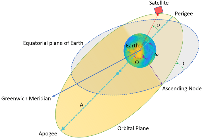
GPS satellites revolve around the Earth in an elliptical orbit, with Earth at one of the focal points of the ellipse. A set of orbital parameters that accurately defines a satellite position in this elliptical orbit is called ephemeris. Each GPS satellite transmits its own ephemeris data on subframes 2 and 3 for LNAV data and on message types 10 and 11 for CNAV data. This figure shows five orbital parameters for a satellite in the Earth-centered Earth-fixed (ECEF) coordinate system. This figure does not show an actual GPS satellite, and the figure is for illustration only.
Length of semimajor axis, : Distance from the center of the elliptical orbit of the satellite to the apogee or perigee
Inclination angle, : Angle between the equatorial plane of Earth and the plane of the orbit of the satellite
Longitude of ascending node, : Angle between the Greenwich meridian and the direction of the ascending node
Argument of perigee, : Angle between the direction of the ascending node and the direction of the perigee
True anomaly, : Angle between the direction of the perigee and the direction of the current position of the satellite
Per Kepler's second law of planetary motion, the angular velocity (rate of change of true anomaly) is different at different locations in the orbit. You can define the mean anomaly, whose rate of change is constant over the entire orbit of the satellite. In GPS ephemeris parameters, rather than specifying true anomaly, mean anomaly is specified (from which true anomaly can be found). IS-GPS-200L Table 20-IV [1] specifies the algorithms that relate mean anomaly and true anomaly.
The eccentricity of the ellipse also defines the orbit. Eccentricity gives a measure of deviation of the elliptical orbit from the circular shape.
A similar set of properties exist for the LNAV data. Create a configuration object to store the LNAV data.
lnavConfig = HelperGPSNavigationConfig(SignalType = "LNAV", PRNID = PRNID)lnavConfig =
HelperGPSNavigationConfig with properties:
SignalType: "LNAV"
PRNID: 1
FrameIndices: [1 2 3 4 5 6 7 8 9 10 11 12 13 14 15 16 17 18 19 20 21 22 23 24 25]
TLMMessage: 0
HOWTOW: 1
AntiSpoofFlag: 0
CodesOnL2: "P-code"
L2PDataFlag: 0
SVHealth: 0
IssueOfDataClock: 0
URAID: 0
WeekNumber: 2149
GroupDelayDifferential: 0
SVClockCorrectionCoefficients: [3×1 double]
ReferenceTimeOfClock: 0
SemiMajorAxisLength: 26560000
MeanMotionDifference: 0
FitIntervalFlag: 0
Eccentricity: 0.0200
MeanAnomaly: 0
ReferenceTimeOfEphemeris: 0
HarmonicCorrectionTerms: [6×1 double]
IssueOfDataEphemeris: 0
IntegrityStatusFlag: 0
ArgumentOfPerigee: -0.5200
RateOfRightAscension: 0
LongitudeOfAscendingNode: -0.8400
Inclination: 0.3000
InclinationRate: 0
AlertFlag: 0
AgeOfDataOffset: 0
NMCTAvailabilityIndicator: 0
NMCTERD: [30×1 double]
AlmanacFileName: "gpsAlmanac.txt"
Ionosphere: [1×1 struct]
UTC: [1×1 struct]
TextMessage: 'This content is part of Satellite Communications Toolbox. Thank you. '
GPS Signal Generation
To generate a GPS signal at the baseband, follow these steps.
Generate the navigation data bits at 50 bits per second.
Based on the configuration, generate C/A-code, P-code, L2 CM-/L2 CL-code, or a combination (happens inside gpsWaveformGenerator object).
Spread the CNAV or LNAV data bit with the appropriate ranging codes (happens inside gpsWaveformGenerator object).
Map the bits on both of the branches as bit 0 to +1 and bit 1 to –1 (happens inside gpsWaveformGenerator object).
Collect data for the in-phase branch and quadrature-phase branch by rate-matching the codes in each branch (happens inside gpsWaveformGenerator object).
(Optional) Write this baseband waveform to a file (depending on the
writeWaveformToFileproperty value).
Based on the configuration, generate the CNAV data.
cnavDataFull = HelperGPSNAVDataEncode(cnavConfig);
Pass the CNAV data through the convolutional encoder.
% Initialize the trellis for convolutional encoder
trellis = poly2trellis(7,["1+x+x^2+x^3+x^6" "1+x^2+x^3+x^5+x^6"]);
cenc = comm.ConvolutionalEncoder(TrellisStructure = trellis, ...
    TerminationMethod = "Continuous");
encodedCNAVData = cenc(cnavDataFull);
Based on the configuration, generate the LNAV data.
lnavDataFull = HelperGPSNAVDataEncode(lnavConfig);
The generated LNAV data and CNAV data contains many bits. Of them choose the data bits based on NavDataBitStartIndex and NumNavDataBits.
dataBitIdx = NavDataBitStartIndex + (0:NumNavDataBits-1);
lnavData = logical(lnavDataFull(dataBitIdx));
cnavData = logical(encodedCNAVData(dataBitIdx));
Specify all of the required properties for waveform generation and create gpsWaveformGenerator object.
% Initialize the GPS waveform generation object
gpswaveobj = gpsWaveformGenerator(SignalType=signalType, ...
    PRNID=PRNID, ...
    SampleRate=sampleRate, ...
    EnablePCode=true, ...
    HasDataWithCACode=hasDataWithCACode, ...
    HasDataWithPCode=hasDataWithPCode)
gpswaveobj =
  gpsWaveformGenerator with properties:

           SignalType: "legacy"
                PRNID: 1
          EnablePCode: true
     HasDataWithPCode: true
    HasDataWithCACode: true
          InitialTime: 0
           SampleRate: 40920000

  Show all properties
bitDuration = gpswaveobj.BitDuration; % BitDuration is a read-only property that gets its value based on SignalType

% Assuming the simulation starts at the beginning of the week, calculate
% the initial time based on navigation data start index.
inittow = bitDuration*(NavDataBitStartIndex-1);
gpswaveobj.InitialTime = inittow;
Create a file into which the waveform is written.
if writeWaveformToFile == 1
    bbWriter = comm.BasebandFileWriter("Waveform.bb",sampleRate,0);
end
Generate the GPS waveform by passing the navigation data through the gpsWaveformGenerator object.
gpsBBWaveform = gpswaveobj({lnavData,cnavData});
size(gpsBBWaveform)
ans = 1×2
818400 1
Optionally write the generated waveform to a file.
if writeWaveformToFile == 1
    bbWriter(gpsBBWaveform);
    release(bbWriter);
end
Signal Visualization
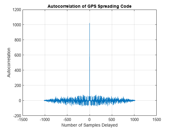
Plot auto-correlation of the C/A-code. Auto-correlation of the ranging code sequence is near-zero except at zero delay, and cross-correlation of two different sequences is near-zero. Because the C/A-code is periodic with a period of 1023 chips, auto-correlation has a peak for a delay of every 1023 chips.
if showVisualizations
    IBranchData = real(gpsBBWaveform);
    QBranchData = imag(gpsBBWaveform);
    corrdata = QBranchData(1:1e-3*sampleRate,1); % Auto-correlate with 1 millisecond of data
    lags = linspace(-1023,1023,2*size(corrdata,1)-1);
    plot(lags,xcorr(corrdata))
    grid on
    xlabel("Number of C/A-code chips Delayed")
    ylabel("Autocorrelation")
    title("Autocorrelation of GPS Spreading Code")
end
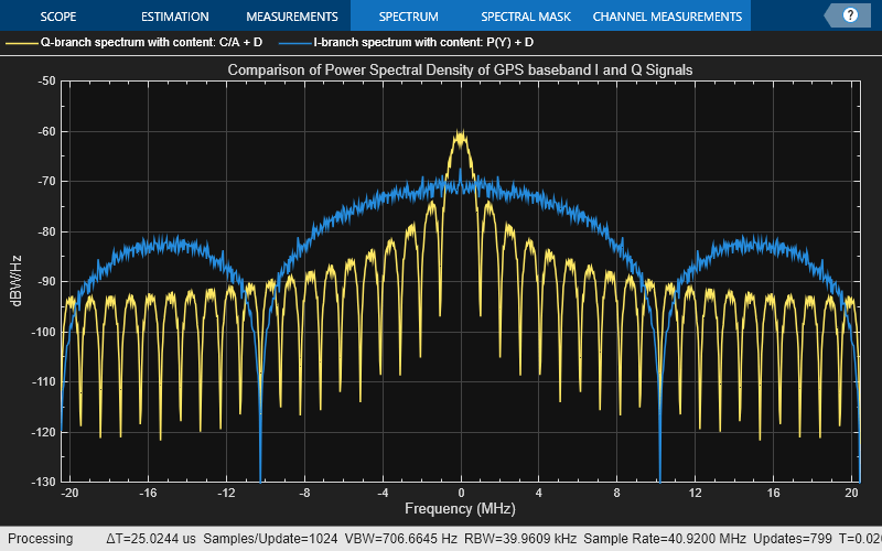
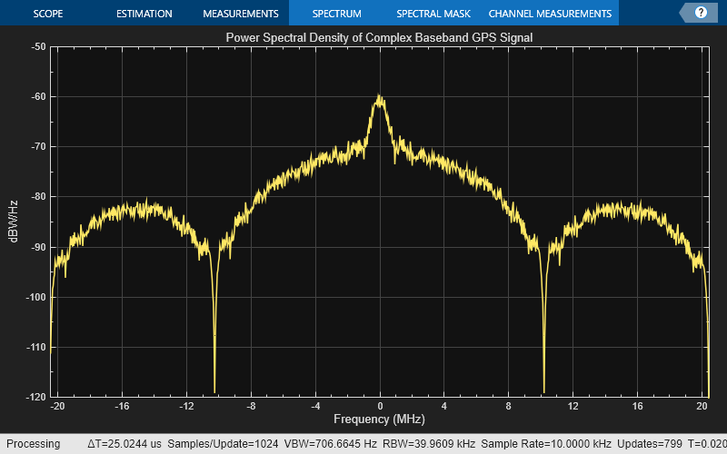
Compare the power spectral density of in-phase branch and quadrature-branch signals. This spectrum plot shows that the P-code is wider when P-code is used.
if showVisualizations
    if hasDataWithPCode == true
        IBranchContent = "P(Y) + D";
    else
        IBranchContent = "P(Y)";
    end

    if signalType == "l2c"
        QBranchContent = "L2 CM + Dc With L2 CL";
    else % legacy
        if hasDataWithCACode ==true
            QBranchContent = "C/A + D";
        else
            QBranchContent = "C/A";
        end
    end

    % Plot the power spectral density of the in-phase and quadrature-phase
    % signals separately
    iqScope = spectrumAnalyzer(SampleRate = sampleRate, ...
        SpectrumType = "Power density", ...
        SpectrumUnits = "dBW", ...
        YLimits = [-130, -50], Title = ...
        "Comparison of Power Spectral Density of GPS baseband I and Q Signals", ...
        ShowLegend = true, ChannelNames = ...
        ["Q-branch spectrum with content: " + QBranchContent, ...
        "I-branch spectrum with content: " + IBranchContent]);

    iqScope([QBranchData,IBranchData]);

    % Plot the signal power spectral density of the entire baseband signal
    bbscope = spectrumAnalyzer(SampleRate = sampleRate, ...
        SpectrumType = "Power density", ...
        SpectrumUnits = "dBW", ...
        YLimits = [-120,-50], ...
        Title = "Power Spectral Density of Complex Baseband GPS Signal");
    bbscope(gpsBBWaveform);
end
Further Exploration
Generate more GNSS waveforms — You can generate any GPS waveform by using
gpsWaveformGeneratorSystem object™. For more information on GPS L1C, NavIC, and Galileo waveforms, see the GPS L1C Waveform Generation, NavIC Waveform Generation, and Galileo Waveform Generation examples respectively.Transmit over-the-air using SDR — To generate GPS waveforms from satellite scenario and transmit them over-the-air, see the GNSS Signal Transmission Using Software-Defined Radio example.
Design receivers — Use the
gnssSignalAcquirerandgnssSignalTrackerSystem objects to acquire and track GNSS waveforms at the receiver. For step-by-step details on the GPS receiver process, see the GPS Legacy Navigation Receiver Positioning Using C/A-Code example.
Supporting Files
This example uses these helper files:
HelperGPSNAVDataEncode.m— Encode navigation data into bits from data that is in configuration objectHelperGPSNavigationConfig.m— Create configuration object for GPS navigation data
Bibliography
[1] IS-GPS-200, Rev: N. NAVSTAR GPS Space Segment/Navigation User Segment Interfaces. Aug 22, 2022; Code Ident: 66RP1.