Optical Satellite Communication Link Budget Analysis

Open Live Script

This example shows how to analyze the link budget for optical communication inter-satellite link, uplink, and downlink. Optical satellite communication provides the advantage of larger bandwidth, a license-free spectrum, higher data rate, and lower power consumption compared to radio frequency-based satellite communication. The link budget calculation for uplink and downlink in this example includes the atmospheric effects due to absorption and scattering.

Set Optical Link Parameters

The performance of an optical communication system is commonly evaluated in terms of link margin. A positive link margin indicates that the link has enough power to overcome the attenuation. A negative link margin indicates that the received signal is too weak to function properly. To compute the link margin in dB, use this equation:

${LM = P}_{rx} - P_{req}$ ,

where:

$P_{rx}$ is the received signal power in dBm.
$P_{req}$ is the required signal power to achieve a specific bit error rate (BER) at a given data rate in dBm.

This example considers the receiver sensitivity as —35.5 dBm for on-off keying modulation with a 10 Gbps data rate and $10^{- 12}$ BER, as defined in [4].

Preq = -35.5; % Required signal power in dBm
Ptx = 17.5;   % Transmitted power in dBm

% Configure the ground station, satellites, and link characteristics
% Set the ground station characteristics with parabolic telescope
gs = struct;
gs.Height = 1;                % Height above the mean sea level in km
gs.OpticsEfficiency = 0.8;    % Optical antenna efficiency
gs.ApertureDiameter = 1;      % Antenna aperture diameter in m
gs.PointingError = 1e-6;      % Pointing error in rad

% Set the satellite A characteristics with parabolic telescope
satA = struct;
satA.Height = 550;            % Height above the mean sea level in km
satA.OpticsEfficiency = 0.8;  % Optical antenna efficiency
satA.ApertureDiameter = 0.07; % Antenna aperture diameter in m
satA.PointingError = 1e-6;    % Pointing error in rad

% Set the satellite B characteristics with parabolic telescope
satB = struct;
satB.OpticsEfficiency = 0.8;  % Optical antenna efficiency
satB.ApertureDiameter = 0.06; % Antenna aperture diameter in m
satB.PointingError = 1e-6;    % Pointing error in rad

% Set the link characteristics
link = struct;
link.Wavelength = 1550e-9;    % m
link.TroposphereHeight = 20;  % km (Typically ranges from 6-20 km)
link.ElevationAngle = 50;     % degrees
link.SatDistance = 1000;      % Distance between satellites in km
link.Type = "downlink";       % "downlink"|"inter-satellite"|"uplink"
% When the Type field is set to "uplink" or "downlink", you must specify
% the CloudType field, as defined in [5] table 1
link.CloudType = "Thin cirrus";

Analyze Link Budget

Analyze the link budget for communication over the optical inter-satellite link, uplink, or downlink, depending on the value of the Type field of the link structure. For uplink and downlink, the optical link is between the ground station and satellite A. The inter-satellite link is between satellite A and satellite B. By default, this example calculates the link budget for downlink.

if link.Type=="downlink"
    % satellite A to ground station
    tx = satA;
    rx = gs;
elseif link.Type=="uplink"
    % Ground station to satellite A
    tx = gs;
    rx = satA;
else % "inter-satellite"
    % satellite A to satellite B
    tx = satA;
    rx = satB;
end

Link Budget for Inter-Satellite Link

An optical inter-satellite link is the link between two satellites. In this case, satellite A and satellite B. The propagation medium is the vacuum of space. To compute the received power for an optical inter-satellite link in dBm, use this equation:

$P_{rx} = P_{tx} + {OE}_{tx} + {OE}_{rx} + G_{tx} + G_{rx} - {LP}_{tx} - {LP}_{rx} - L_{PS}$ ,

where:

$P_{tx}$ is the transmitted power in dBm.
${OE}_{tx}$ is the transmitter optical efficiency in dB.
${OE}_{rx}$ is the receiver optical efficiency in dB.
$G_{tx}$ is the transmitter gain in dB.
$G_{rx}$ is the receiver gain in dB.
${LP}_{tx}$ is the transmitter pointing loss in dB.
${LP}_{rx}$ is the receiver pointing loss in dB.
$L_{PS}$ is the free-space path loss between the two satellites in dB.

Transmitter and receiver pointing loss, as defined in [4], is

${LP}_{tx} = 4.3429 {\times g}_{tx} {\times ({Pe}_{tx})}^{2}$ ,

${LP}_{rx} = 4.3429 \times {g_{rx} \times ({Pe}_{rx})}^{2}$ ,

where:

${Pe}_{tx}$ is the transmitter pointing error in radians.
$g_{tx}$ is the transmitter linear gain.
${Pe}_{rx}$ is the receiver pointing error in radians.
$g_{rx}$ is the receiver linear gain.

Transmitter and receiver gain in dB, is

$G_{tx} = 10 {\times \log}_{10} (g_{tx})$ ,

$G_{rx} = 10 {\times \log}_{10} (g_{rx})$ ,

Use the following equations, as defined in ITU-R S.1590 Section 5.1 [1], to calculate $g_{tx}$ and $g_{rx}$ :

$g_{tx} = {(\frac{π d_{tx}}{λ})}^{2}$ ,

$g_{rx} = {(\frac{π d_{rx}}{λ})}^{2}$ ,

where:

$λ$ is the wavelength in m.
$d_{tx}$ is the diameter of the primary aperture of the transmitter antenna in m.
$d_{rx}$ is the diameter of the primary aperture of the receiver antenna in m.

% Calculate transmitter and receiver gain
txGain = (pi*tx.ApertureDiameter/link.Wavelength)^2;
Gtx = 10*log10(txGain); % in dB
rxGain = (pi*rx.ApertureDiameter/link.Wavelength)^2;
Grx = 10*log10(rxGain); % in dB
% Calculate transmitter and receiver pointing loss in dB
txPointingLoss = 4.3429*(txGain*(tx.PointingError)^2);
rxPointingLoss = 4.3429*(rxGain*(rx.PointingError)^2);

% Calculate link margin for inter-satellite link in dB
if link.Type=="inter-satellite"
    % Free-space path loss between satellites in dB
    pathLoss = fspl(link.SatDistance*1e3,link.Wavelength);
    linkMargin = Ptx + 10*log10(tx.OpticsEfficiency) + 10*log10(rx.OpticsEfficiency) + ...
        Gtx + Grx - txPointingLoss - rxPointingLoss - pathLoss - Preq;
    disp("Link margin for inter-satellite link is "+num2str(linkMargin)+" dB")
end

Link Budget for Uplink and Downlink

For an optical uplink and downlink, the optical beams go through the atmosphere causing attenuation due to absorption and scattering. To compute the received power for an optical uplink or downlink in dB, use this equation:

$P_{r} = P_{tx} + {OE}_{tx} + {OE}_{rx} + G_{tx} + G_{rx} - {LP}_{tx} - {LP}_{rx} - L_{PG} - L_{abs} - L_{sca}$ ,

where:

$L_{PG}$ is the free-space path loss between the ground station and satellite in dB.
$L_{abs}$ is the atmospheric attenuation loss due to absorption in dB.
$L_{sca}$ is the atmospheric attenuation loss due to scattering in dB.

Free-space path loss, as defined in ITU-R S.1590 Section 5.1 [1], is

$L_{PG} = 20 {\times \log}_{10} (\frac{λ}{4 π d_{GS}})$ ,

where $d_{GS}$ is the distance between the ground station and satellite. Assuming the satellite is moving in a circular orbit, compute $d_{GS}$ using slantRangeCircularOrbit function.

Atmospheric Attenuation for Uplink and Downlink

Absorption and scattering of atmospheric molecules and aerosols affect free-space optical propagation. The absorptive characteristics of the atmosphere above 10 THz are favorable for propagation. This example considers a wavelength of 1550 nm, which has low absorption characteristics, as specified in ITU-R P.1621-2 figure 2 [2]. This example considers an absorption loss of 0.01 dB.

absorptionLoss = 0.01; % Absorption loss in dB

Aerosol particles and water droplets present along the propagation path cause atmospheric scattering. Scattering causes redirection of the transmitted energy away from the intended propagation path. This redirection of energy results in an apparent reduction in signal strength at the receiver. Total scattering loss in dB is

$L_{sca} = L_{geo} + L_{mie}$ ,

where:

$L_{geo}$ is the attenuation due to geometrical scattering in dB.
$L_{mie}$ is the attenuation due to Mie scattering in dB.

Geometrical scattering occurs due to fog or dense clouds. The atmosphere exhibits geometrical scattering when the size of the particles along the propagation path is much greater than the signal wavelength. The attenuation due to geometrical scattering, in dB, using Beers-Lambert law as defined in [5], is

$L_{geo} = 4.3429 \times A_{geo} \times d_{T}$ ,

where:

$A_{geo}$ is the attenuation coefficient due to geometrical scattering.
$d_{T}$ is the distance of the optical beam that propagates through the troposphere layer of the atmosphere.

To compute the attenuation coefficient due to geometrical scattering, use this equation:

$A_{geo} = \frac{3.91}{V} \times {(\frac{λ}{550})}^{- δ}$ ,

where:

$V$ is the visibility in km.
$δ$ is the particle size coefficient.

Mie scattering occurs due to the scattering of light by aerosols. The atmosphere exhibits Mie scattering characteristics when the particles along the propagation path have the same diameter as the signal wavelength. It mainly occurs in the lower part of the atmosphere. Atmospheric attenuation due to Mie scattering, in dB, as defined in ITU-R P.1622-1 Section 3.1 [3], is

$L_{mie} = \frac{{4.3429 \times ER}_{mie}}{\sin (θ_{E})}$ ,

where ${ER}_{mie}$ is the extinction ratio for Mie scattering.

To calculate the Mie scattering extinction ratio, use this equation:

${ER}_{mie} = a {h_{GS}}^{3} + b {h_{GS}}^{2} + c h_{GS} + d$ ,

where:

$a = 0.000487 λ^{3} - 0.002237 λ^{2} + 0.003864 λ - 0.004442$
$b = - 0.00573 λ^{3} + 0.02639 λ^{2} - 0.04552 λ + 0.05164$
$c = 0.02565 λ^{3} - 0.1191 λ^{2} + 0.20385 λ - 0.216$
$d = - 0.0638 λ^{3} + 0.3034 λ^{2} - 0.5083 λ + 0.425$

This method is appropriate for ground stations with elevations between 0 and 5 km above sea level and wavelengths between 800 and 2000 nm. This method is accurate to within approximately 0.1 dB for an elevation angle greater than 45º.

% Calculate link margin for uplink or downlink
if (link.Type=="uplink") || (link.Type=="downlink")

    % Calculate the distance of the optical beam that propagates through
    % the troposphere layer of the atmosphere in km
    dT = (link.TroposphereHeight - gs.Height).*cscd(link.ElevationAngle);

    % Calculate the slant distance for uplink and downlink between
    % satellite A and the ground station for circular orbit in m
    dGS = slantRangeCircularOrbit(link.ElevationAngle,satA.Height*1e3,gs.Height*1e3);

    % Calculate free-space path loss between the ground station and
    % satellite in dB
    pathLoss = fspl(dGS,link.Wavelength);       

    % Calculate loss due to geometrical scattering
    % cnc - cloud number concentration in cm-3
    % lwc - Liquid water content in g/m-3
    [cnc,lwc] = getCloudParameters(link.CloudType); 
    visibility = 1.002/((lwc*cnc)^0.6473);                   % Calculate visibility in km
    % Get particle size related coefficient
    if visibility<=0.5
        delta = 0;
    elseif visibility>0.5 && visibility<=1
        delta = visibility - 0.5;
    elseif visibility>1 && visibility<=6
        delta = 0.16*visibility + 0.34;
    elseif visibility>=6 && visibility<=50
        delta = 1.3;
    else                                                     % visibility>50
        delta = 1.6;
    end
    geoCoeff = (3.91/visibility)* ...
        ((link.Wavelength*1e9/550)^-delta);                  % Extinction coefficient
    geoScaLoss = 4.3429*geoCoeff*dT;                         % Geometrical scattering loss in dB

    % Calculate loss due to Mie scattering
    lambda_mu = link.Wavelength*1e6;                         % Wavelength in microns
    % Calculate empirical coefficients
    a = (0.000487*(lambda_mu^3)) - (0.002237*(lambda_mu^2)) + ...
        (0.003864*lambda_mu) - 0.004442;
    b = (-0.00573*(lambda_mu^3)) + (0.02639*(lambda_mu^2)) - ...
        (0.04552*lambda_mu) + 0.05164;
    c = (0.02565*(lambda_mu^3)) - (0.1191*(lambda_mu^2)) + ...
        (0.20385*lambda_mu) - 0.216;
    d = (-0.0638*(lambda_mu^3)) + (0.3034*(lambda_mu^2)) - ...
        (0.5083*lambda_mu) + 0.425;
    mieER = a*(gs.Height^3) + b*(gs.Height^2) + ...
    c*(gs.Height) + d;                                       % Extinction ratio
    mieScaLoss = (4.3429*mieER)./sind(link.ElevationAngle);  % Mie scattering loss in dB

    % Calculate link margin for uplink or downlink in dB
    linkMargin = Ptx + 10*log10(tx.OpticsEfficiency) + ...
        10*log10(rx.OpticsEfficiency) + Gtx + Grx - ...
        txPointingLoss - rxPointingLoss - pathLoss - ...
        absorptionLoss - geoScaLoss - mieScaLoss - Preq;                                    
    disp("Link margin for "+num2str(link.Type)+" is "+num2str(linkMargin)+" dB")
end

Link margin for downlink is 6.6377 dB

Further Exploration

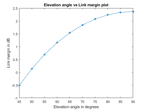
This figure plots the elevation angle versus the link margin for this example with Ptx = 11 dBm, and the ElevationAngle field of the link structure varying from 45 to 90 degrees. The plot shows that the link margin increases with the increase in the elevation angle.

Try running this example with these modifications

Observe the link margin for uplink and inter-satellite link.
Observe the link margin and geometrical scattering loss for different cloud types.
Observe the link margin by varying any property of the ground station, satellite, or link.

References

[1] International Telecommunication Union Radiocommunication Sector (ITU-R). Technical and operational characteristics of satellites operating in the range 20-375 THz. Recommendation ITU-R S.1590 (09/2022). https://www.itu.int/rec/R-REC-S.1590-0-200209-I/en.

[2] International Telecommunication Union Radiocommunication Sector (ITU-R). Propagation data required for the design of Earth-space systems operating between 20 THz and 375 THz. Recommendation ITU-R P.1621-2 (07/2015). https://www.itu.int/rec/R-REC-P.1621-2-201507-I/en.

[3] International Telecommunication Union Radiocommunication Sector (ITU-R). Prediction methods required for the design of Earth-space systems operating between 20 THz and 375 THz. Recommendation ITU-R P.1622-1 (08/2022). https://www.itu.int/rec/R-REC-P.1622-1-202208-I/en.

[4] Liang, Jintao, Aizaz U. Chaudhry, Eylem Erdogan, and Halim Yanikomeroglu. “Link Budget Analysis for Free-Space Optical Satellite Networks.” In 2022 IEEE 23rd International Symposium on a World of Wireless, Mobile and Multimedia Networks (WoWMoM), 471–76. Belfast, United Kingdom: IEEE, 2022. https://doi.org/10.1109/WoWMoM54355.2022.00073.

[5] Awan M. S., Marzuki, E. Leitgeb, B. Hillbrand, F. Nadeem, and M. S. Khan, "Cloud Attenuations for Free-Space Optical Links." 2009 International Workshop on Satellite and Space Communications, 274-8. Siena, Italy: IEEE, https://doi.org/10.1109/IWSSC.2009.5286364.

Local Functions

getCloudParameters — Gets the gamma distribution parameters for different clouds, as defined for the selected cloudType in [5] table 1.

function [cnc,lwc] = getCloudParameters(cloudType)
% cnc - Cloud number concentration in 1/cm^3
% lwc - Liquid water content g/m^3
switch cloudType
    case "Cumulus"
        cnc = 250;
        lwc = 1;
    case  "Stratus"
        cnc = 250;
        lwc = 0.29;
    case "Stratocumulus"
        cnc = 250;
        lwc = 0.15;
    case "Altostratus"
        cnc = 400;
        lwc = 0.41;
    case "Nimbostratus"
        cnc = 200;
        lwc = 0.65;
    case "Cirrus"
        cnc = 0.025;
        lwc = 0.06405;
    case "Thin cirrus"
        cnc = 0.5;
        lwc = 3.128*1e-4;
end
end