Wind Turbine Blade Optimization

Open Live Script

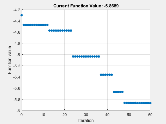
This example shows how to adjust the twist and chord length along a wind turbine blade to optimize power output. It combines a Simscape™ Driveline™ test harness model with the fminsearch optimization function. The wind turbine model uses blade element momentum (BEM) theory, including wake rotation. By putting the test harness into Fast Restart, you can enable rapid optimization iterations. In this case, the optimization increases the power output from 4.3 MW to 5.9 MW. Other products available for performing this type of optimization with Simscape Driveline models include the Optimization Toolbox™ and Simulink® Design Optimization™. These products provide predefined functions to manipulate and analyze blocks using either GUIs or a command line approach.

Create the Test Harness

model = 'WindTurbineBladeOptimization';
open_system(model);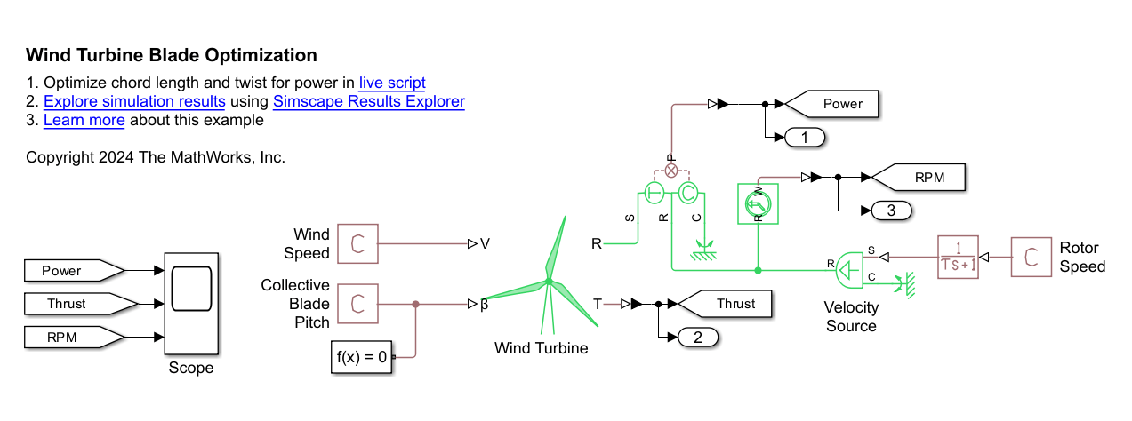

The test harness applies a steady wind speed and maintains the collective blade pitch at 0 deg. To expedite iterations, the model excludes the rotor inertia and a more detailed driveline. The Velocity Source absorbs the generated power. For numerical robustness when iterating over parameters in the relatively stiff test harness, the rotor starts from rest and gradually ramps up to the target rotor speed over 5 seconds. Fast Restart mode avoids recompiling the model between iterations, further speeding up the optimization process. The Wind Turbine block outputs a thrust measurement, while sensors measure the rotor speed and power.

Define Fixed Parameters

This example sets the turbine diameter at 126 meters, rated wind speed at 11.4 m/s, and target tip speed ratio at 7. The tip speed ratio is defined as

$λ = \frac{R Ω}{V_{Wind}}$

where:

$R$ is the rotor radius.
$Ω$ is the rotor angular velocity.
$V_{Wind}$ is the incident air velocity.

Design.rotorDiameter = 126;                    % [m]
Design.rotorRadius = Design.rotorDiameter / 2; % [m]
Design.TSRtarget = 7;                          % [-]
Harness.windSpeed = 11.4; % [m/s]
Harness.rotorSpeed = Design.TSRtarget * Harness.windSpeed / Design.rotorRadius * 60/(2*pi); % [rpm]

This example also fixes the air foil type distribution along the blades. The distribution is based on the report by Jason Jonkman, “Definition of a 5-MW Reference Wind Turbine for Offshore System Development.” National Renewable Energy Lab (NREL), Golden, CO (United States), No. NREL/TP-500-38060 (2009). This airfoil distribution matches the default parameters of the Wind Turbine block.

Radial Location Normalized by Rotor Radius	Airfoil Name
0.11	Round root with Cd = 0.35
0.17	DU40 airfoil with aspect ratio of 17
0.23	DU35 airfoil with aspect ratio of 17
0.37	DU30 airfoil with aspect ratio of 17
0.5	DU25 airfoil with aspect ratio of 17
0.63	DU21 airfoil with aspect ratio of 17
1	NACA64 airfoil with aspect ratio of 17

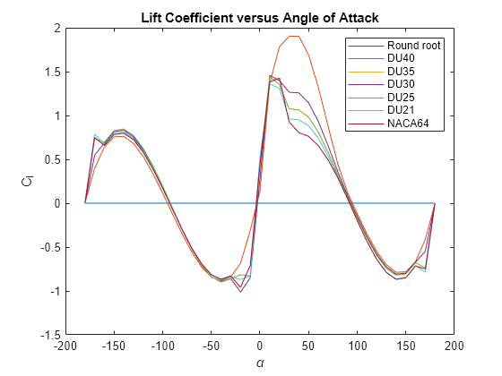
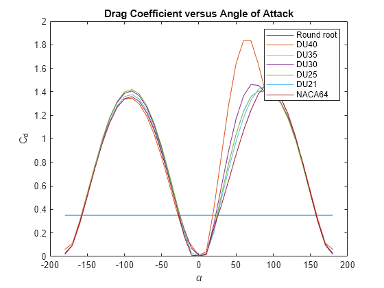
Retrieve and plot the block's airfoil data.

blk = [model '/Wind Turbine'];
Data.radius_TLU = eval( get_param(blk, 'radial_TLU') ) * Design.rotorRadius; % [m]
Data.alpha_TLU = eval( get_param(blk, 'alpha_TLU') );                        % [deg]
Data.Cl_TLU = eval( get_param(blk, 'Cl_TLU') );                              % [-]
Data.Cd_TLU = eval( get_param(blk, 'Cd_TLU') );                              % [-]

figure;
plot(Data.alpha_TLU, Data.Cl_TLU);
title('Lift Coefficient versus Angle of Attack')
xlabel('\alpha')
ylabel('C_l')
legend('Round root', 'DU40', 'DU35', 'DU30', 'DU25', 'DU21', 'NACA64');

Figure contains an axes object. The axes object with title Lift Coefficient versus Angle of Attack, xlabel alpha, ylabel C indexOf l baseline C_l contains 7 objects of type line. These objects represent Round root, DU40, DU35, DU30, DU25, DU21, NACA64.

figure;
plot(Data.alpha_TLU, Data.Cd_TLU);
title('Drag Coefficient versus Angle of Attack')
xlabel('\alpha')
ylabel('C_d')
legend('Round root', 'DU40', 'DU35', 'DU30', 'DU25', 'DU21', 'NACA64')

Figure contains an axes object. The axes object with title Drag Coefficient versus Angle of Attack, xlabel alpha, ylabel C indexOf d baseline C_d contains 7 objects of type line. These objects represent Round root, DU40, DU35, DU30, DU25, DU21, NACA64.

Calculate Initial Values for Twist and Chord Length

For an ideal blade without wake rotation or drag, the optimal twist and chord length along the blades is

$ϕ_{Opt} = \tan^{- 1} (\frac{2}{3 λ_{r}})$

$ϕ_{Opt} = θ_{T, Opt} + α_{Opt}$

$c_{Opt} = \frac{8 π r}{{BC}_{l, Opt}} (\frac{\sin ϕ_{Opt}}{3 λ_{r}})$

where

$r$ is the radial location.
$λ_{r} = λ \frac{r}{R}$ is the speed ratio at the radial location.
$ϕ_{Opt}$ is the optimal angle of relative wind.
$θ_{T, Opt}$ is the optimal twist.
$α_{Opt}$ is the angle of attack where Cd/Cl is minimal.
$C_{l, Opt}$ is the lift coefficient at the optimal angle of attack.
$c_{Opt}$ is the optimal chord length.
$B = 3$ is the number of blades in the rotor.

These expressions are derived in Manwell, J. F., J. G. McGowan, and A. L. Rogers. Wind Energy Explained: Theory, Design and Application. 1st ed. Wiley. 2009.

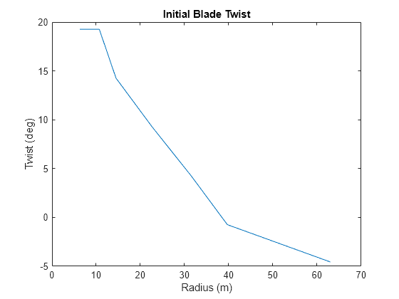
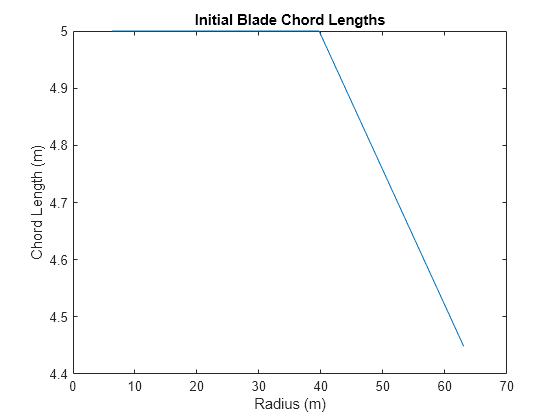
For the chosen airfoils, the ratio of drag coefficient to lift coefficient (Cd/Cl) is minimal at an angle of attack of 10 deg. This example optimizes the blade chord length and twist angle at six radial locations. To ensure a smooth aerodynamic surface and maintain structural integrity, the optimization constrains all chord lengths to be between 1.5 and 5 meters and limits the change in twist between radial sections to less than 5 deg.

Calculate and plot the initial values for twist and chord length along the blades.

Opt.Init.alpha = 10 * pi / 180; % Initial value for angle of attack [rad]
Design.B = 3;                   % Number of blades [-]

Opt.numRadialLocationsToOptimize = 6; % Number of radial sections to optimize

% Initialize vectors
Opt.Init.twist = zeros(1, Opt.numRadialLocationsToOptimize); % Vector of initial value for twist [deg]
Opt.Init.chord = zeros(1, Opt.numRadialLocationsToOptimize); % Vector of initial value for chord length [m]

for i=1:Opt.numRadialLocationsToOptimize
    Opt.Init.r        = Data.radius_TLU(i+1);
    Opt.Init.lambda_r = Design.TSRtarget * Opt.Init.r / Design.rotorRadius; % Local tip speed ratio [-]
    Opt.Init.phi      = atan(2 / (3 * Opt.Init.lambda_r) ); % Angle of relative twist [rad]
    Opt.Init.twist(i) = 180 / pi * (Opt.Init.phi - Opt.Init.alpha); % [deg]

    Opt.Init.Cl       = interp1(Data.alpha_TLU, Data.Cl_TLU(:,i), Opt.Init.alpha); % Lift coefficient [-]
    Opt.Init.chord(i) = 8 * pi * Opt.Init.r * sin(Opt.Init.phi) / (Design.B * Opt.Init.Cl * 3 * Opt.Init.lambda_r); % [m]
end

% Set twist at round root equal to neighboring twist
Opt.Init.twist = [Opt.Init.twist(1) Opt.Init.twist];

% Adjust twist based on maximum permitted change in twist between radial sections
Design.twistMaxDiff = 5; % Maximum permitted change in twist between radial sections [deg]
for i = 2:length(Opt.Init.twist)
    if Opt.Init.twist(i) > Opt.Init.twist(i-1) + Design.twistMaxDiff
        Opt.Init.twist(i) = Opt.Init.twist(i-1) + Design.twistMaxDiff;
    elseif Opt.Init.twist(i) < Opt.Init.twist(i-1) - Design.twistMaxDiff
        Opt.Init.twist(i) = Opt.Init.twist(i-1) - Design.twistMaxDiff;
    end
end

% Limits to chord
Design.chordMax = 5;    % Maximum permitted chord length [m]
Design.chordMin = 1.5;  % Minimum permitted chord length [m]

% Assign maximum permitted chord to the root
Opt.Init.chord = [Design.chordMax Opt.Init.chord];

% Limit the chord lengths
Opt.Init.chord(Opt.Init.chord > Design.chordMax) = Design.chordMax;
Opt.Init.chord(Opt.Init.chord < Design.chordMin) = Design.chordMin;

% Plot the initial twist and chord lengths
figure;
plot(Data.radius_TLU, Opt.Init.twist);
ylabel('Twist (deg)');
xlabel('Radius (m)');
title('Initial Blade Twist');

Figure contains an axes object. The axes object with title Initial Blade Twist, xlabel Radius (m), ylabel Twist (deg) contains an object of type line.

figure;
plot(Data.radius_TLU, Opt.Init.chord);
ylabel('Chord Length (m)');
xlabel('Radius (m)');
title('Initial Blade Chord Lengths');

Figure contains an axes object. The axes object with title Initial Blade Chord Lengths, xlabel Radius (m), ylabel Chord Length (m) contains an object of type line.

Run the Optimization

Since blade element momentum theory does not include a radial component of fluid flow, airflow through each radial section is independent. This allows twist and chord length at each section to be optimized independently. To expedite the optimization process, this example optimizes the twist and chord length of all sections simultaneously. To further speed up the optimization, the model uses Fast Restart mode and the Wind Turbine Blade twist vector, θ_tw(r) and Normalized chord length vector, c(r)/R are run-time parameters. These settings enable optimization iterations to vary the parameter values without recompiling the model.

The function WindTurbineBladeOptimizationRun defines an objective function. This function runs the test harness and uses the negative of the simulated power as the optimization cost. The fminsearch function tries to minimize the cost, thereby maximizing the wind turbine power. WindTurbineBladeOptimizationRun also limits the change in twist between radial sections and limits the chord length to be between the chosen minimum and maximum values.

The plot below updates during the optimization. The function value represents the negated power value in units of MW at each optimization iteration. The plot shows that the initial power is 4.3 MW and the optimized power reaches 5.9 MW after 60 iterations.

Run the optimization.

set_param(model,'FastRestart','on')

% Call the Optimization functions
[Opt.Final.twist, Opt.Final.chord] = WindTurbineBladeOptimizationRun...
    (Opt.Init.twist, Opt.Init.chord, Design.twistMaxDiff, Design.chordMin, Design.chordMax, model);

Figure Optimization Plot Function contains an axes object. The axes object with title Current Function Value: -5.8689, xlabel Iteration, ylabel Function value contains an object of type scatter.

Plot the Optimized Values of Twist and Chord Length

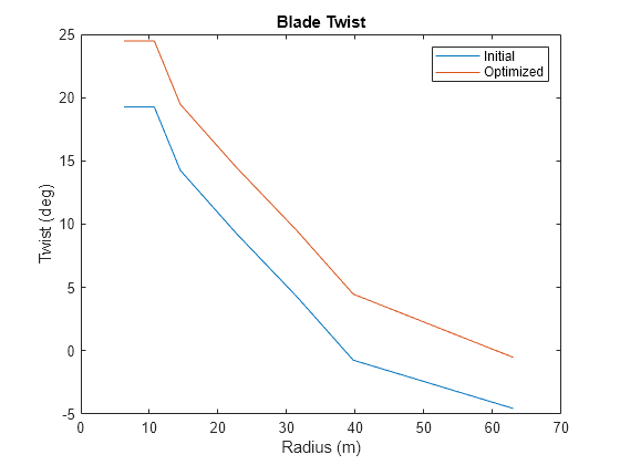
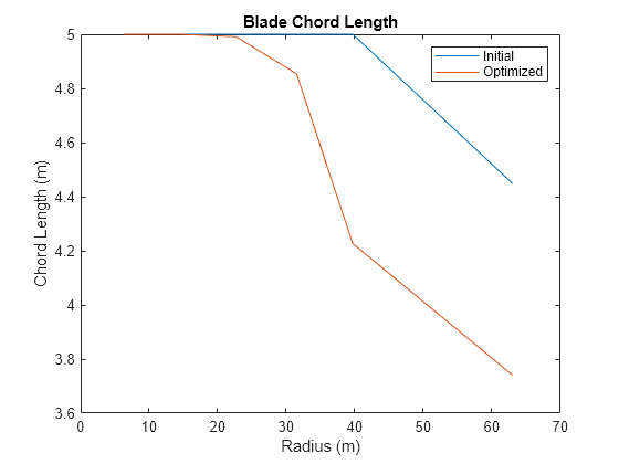
Plot the optimized values of twist and chord length along the blade. Compare these optimized values to the initial values. The optimized blade twist is higher than the initial blade twist. The optimized chord length is smaller than the initial chord length at larger radius locations.

figure;
plot(Data.radius_TLU, Opt.Init.twist, Data.radius_TLU, Opt.Final.twist);
ylabel('Twist (deg)');
xlabel('Radius (m)');
legend('Initial', 'Optimized')
title('Blade Twist');

Figure contains an axes object. The axes object with title Blade Twist, xlabel Radius (m), ylabel Twist (deg) contains 2 objects of type line. These objects represent Initial, Optimized.

figure;
plot(Data.radius_TLU, Opt.Init.chord, Data.radius_TLU, Opt.Final.chord);
ylabel('Chord Length (m)');
xlabel('Radius (m)');
legend('Initial', 'Optimized')
title('Blade Chord Length');

Figure contains an axes object. The axes object with title Blade Chord Length, xlabel Radius (m), ylabel Chord Length (m) contains 2 objects of type line. These objects represent Initial, Optimized.

Generate Power and Thrust Coefficient Plots

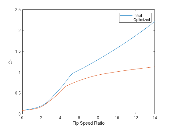
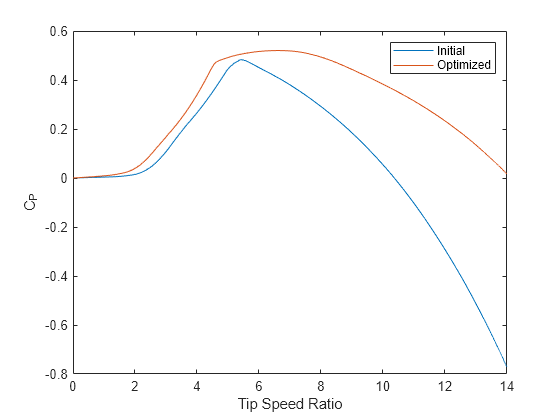
Use the test harness to generate plots of power and thrust coefficient versus tip speed ratio. This allows you to compare the wind turbine performance before and after the optimization. The nondimensional power and thrust coefficients are

$C_{P} = \frac{Power}{0.5 ρ A V_{Wind}^{3}}$

$C_{T} = \frac{Thrust}{0.5 ρ A V_{Wind}^{2}}$

where:

$C_{P}$ is the power coefficient.
$C_{T}$ is the thrust coefficient.
$Power$ is the generated power.
$Thrust$ is the generated thrust.
$ρ$ is the air density.
$A$ is the swept rotor area.
$V_{Wind}$ is the incident air velocity.

The test harness outputs instantaneous power, thrust and rotor speed. Adjust the harness's steady rotor speed to simulate the wind turbine's behavior at higher tip speed ratios. The generated figures show that the optimized wind turbine has a higher power coefficient and lower thrust coefficient for all tip speed ratios.

Harness.rotorSpeed = 2 * Design.TSRtarget * Harness.windSpeed / Design.rotorRadius * 60/(2*pi); % [rpm]

rho = eval( get_param(blk, 'rho_air') ); % Air density [kg/m^3]
Area = pi * Design.rotorRadius^2;        % Rotor swept area [m^2]

% Generate data for initial twist and chord lengths
twist = Opt.Init.twist;
chord = Opt.Init.chord;

out= sim(model);
Opt.Init.power = out.yout(:,1);                    % [MW]
Opt.Init.thrust = out.yout(:,2);                   % [kN]
Opt.Init.rotorSpeed = out.yout(:,3) * 2 * pi / 60; % [rad/s]

Opt.Init.Cp  = Opt.Init.power * 10^6  / (0.5 * rho * Area * Harness.windSpeed^3);
Opt.Init.Ct  = Opt.Init.thrust * 10^3 / (0.5 * rho * Area * Harness.windSpeed^2);
Opt.Init.TSR = Design.rotorRadius * Opt.Init.rotorSpeed / Harness.windSpeed;

% Generate data for optimized twist and chord lengths
twist = Opt.Final.twist;
chord = Opt.Final.chord;

out= sim(model);
Opt.Final.power = out.yout(:,1);                    % [MW]
Opt.Final.thrust = out.yout(:,2);                   % [kN]
Opt.Final.rotorSpeed = out.yout(:,3) * 2 * pi / 60; % [rad/s]

Opt.Final.Cp  = Opt.Final.power * 10^6  / (0.5 * rho * Area * Harness.windSpeed^3);
Opt.Final.Ct  = Opt.Final.thrust * 10^3 / (0.5 * rho * Area * Harness.windSpeed^2);
Opt.Final.TSR = Design.rotorRadius * Opt.Final.rotorSpeed / Harness.windSpeed;

figure;
plot(Opt.Init.TSR, Opt.Init.Cp, Opt.Final.TSR, Opt.Final.Cp);
xlabel('Tip Speed Ratio')
ylabel('C_P')
legend('Initial', 'Optimized');

Figure contains an axes object. The axes object with xlabel Tip Speed Ratio, ylabel C indexOf P baseline C_P contains 2 objects of type line. These objects represent Initial, Optimized.

figure;
plot(Opt.Init.TSR, Opt.Init.Ct, Opt.Final.TSR, Opt.Final.Ct);
xlabel('Tip Speed Ratio')
ylabel('C_T')
legend('Initial', 'Optimized');

Figure contains an axes object. The axes object with xlabel Tip Speed Ratio, ylabel C indexOf T baseline C_T contains 2 objects of type line. These objects represent Initial, Optimized.