CEI-224G-MR Transmitter/Receiver IBIS-AMI Model

Getting Started

The CEI-224G-MR-PAM4 Medium Reach Interface specification (Dec 30, 2024, Contribution Number OIF2024.058.07) was used in the generation of this kit. The parameter values for Channel Operating Margin (COM) are provided in Table 32-1 of the specification.

This example leverages the Simulink model generated from the example ADC IBIS-AMI Model Based on COM, including its attached .m files, as the starting point for building the 224G IBIS-AMI models. You can either complete that example before beginning to build these CEI-224G-MR-PAM4 models or simply open the cei224g_mr_start.slx file included with this example.

Customize Blocks for 224G System in Simulink

Open the provided SerDes Model created from the ADC IBIS-AMI Model Based on COM example.

>> open_system('sim_cei224g_start')

This example updates the data path blocks and adds additional features to support 224G operation.

Note: One of the last steps done in the previous ADC example was to update the Rx model Bits to ignore in the IBIS-AMI Manager to 20,000 before running Export. Since this value is larger than the current setting for Number of symbols in the Stimulus block, no Time Domain results will be output at the end of the simulation. It is recommended that you reduce the Rx model Bits to ignore to 6000 and increase the Number of symbols to 8000 before proceeding.

Configuration Setup

Open the Block Parameter dialog box for the Configuration block and update the settings:

Confirm the following settings remain the same:

Transmitter Model Setup

Open the Tx subsystem. Your canvas should show a FFE and VGA block as follows:

Configure Tx FFE

Open the FFE block mask and change its configuration to have 4 tap weights as follows (Table 32-1):

Confirm the following settings remain the same:

Update Tap Ranges

After changing the number of FFE taps, the tap Min/Max values need to be adjusted per Table 32-3 and 32-6.

Using the IBIS-AMI Manager, update the ranges as follows:

FFE.TapWeights.-2

FFE.TapWeights.-1

FFE.TapWeights.0

FFE.TapWeights.1

Configure Tx VGA

The output swing (T_Vf in Table 32-3) is set using the Tx VGA gain.

Using the IBIS-AMI Manager, update the ranges as follows:

TX_AMP.Gain

Model setup for Tx RLM

Level Separation Mismatch Ratio, commonly known as RLM, is a measure of the irregularity of the various eye openings in a PAMn signal. Per Table 32-1 the Tx RLM should be set to 0.95. For more information about RLM in SerDes toolbox, see Level Separation Mismatch Ratio (RLM) using IBIS-AMI.

Note: Since RLM models non-LTI behavior in the Transmitter, RLM is a GetWave-only feature.

Add a Pass-Through block to the Tx

The first step is to add a Pass-Through block to the Transmitter data path. You will then add a MATLAB function block to the Pass-Through and add code to model the RLM behavior.

To add a new Pass-Through block to the Tx subsystem for RLM:

The Tx subsystem should now look like this:

Edit the Pass-Through block

Next, look under the mask of the RLM_Injection block. Delete the Pass-Through block, then add a MATLAB Function block to the canvas. Edit the MATLAB Function block and replace the entire contents with the following code:

function stimOut = RLM_Injection(stimIn, sign, RLM, Modulation)
% stimOut    Add Transmitter Level MisMatch to incoming stimulus signal.
%            Uses a saturating non-linearity to shift a single symbol
%             voltage on the incoming stimulus waveform.
%            Supports PAMn for N > 2
%            Not valid for NRZ
%
% stimIn     Stimulus input
% sign       Sign of RLM to be added: 1 (positive) or -1 (negative)
% RLM        Ratio of Level MisMatch (RLM) should be between 0.5 and 1.0
%             Only the upper eye is modified by varying the N-1 symbol voltage.
% Modulation Current modulation being used. Passed in via Data Scope = Parameter.
% stimOut    Stimulus output with RLM added.
 
% Copyright 2023 The MathWorks, Inc.
 
% Skip entire function if NRZ
if Modulation == 2
    stimOut = stimIn;
    return
end
 
persistent vinvout
 
if isempty(vinvout)
    % Do not allow RLM smaller than 0.5
    if RLM < 0.5
        RLM = 0.5;
    end
 
    % Determine amount to shift incoming stimulus waveform
    bias = sign*(1-abs(RLM))/(Modulation - 1);
 
    Vswing = 0.5;       %% +/- Input signal swing
    Vstep  = 0.005;     %% Minimum voltage step in Vin/Vout array
 
    % Voltage range to apply bias to
    limit = 0.5/(Modulation - 1);
    % Center of Symbol voltage to be shifted
    Vcent = abs((Vswing * 2)/(Modulation - 1) - Vswing);
  
    % Define incoming voltage points
    vin1 = -Vswing * 2;
    vin2 = -Vswing;
    vin3 =  Vcent - limit/2 - Vstep;
    vin4 =  Vcent - limit/2;
    vin5 =  Vcent;
    vin6 =  Vcent + limit/2;
    vin7 =  Vcent + limit/2 + Vstep + bias;
    vin8 =  Vswing;
    vin9 =  Vswing * 2;
        
    % Define outgoing voltage points
    vout1 = vin1;
    vout2 = vin2;
    vout3 = vin3;
    vout4 = vin4 + bias;
    vout5 = vin5 + bias;
    vout6 = vin6 + bias;
    vout7 = vin7;
    vout8 = vin8;
    vout9 = vin9;
 
    vinvout = [vin1 vout1; vin2 vout2; vin3 vout3; vin4 vout4; vin5 vout5; vin6 vout6; vin7 vout7; vin8 vout8; vin9 vout9];
 
end
 
%% Apply memory-less non-linearity from serdes.SaturatingAmplifier
vin  = vinvout(:,1);
vout = vinvout(:,2);
 
% Perform lookup operation. Inspired by Bentley's binary search in "Programming Pearls".
% Initialize Search Index
lo = 1;
hi = length(vin);
 
if stimIn <= vin(lo)
    stimOut = vout(lo);
elseif stimIn > vin(hi)
    stimOut = vout(hi);
else
    while hi > lo+1
        mid = round((hi+lo)/2);
        if stimIn <= vin(mid)
            hi = mid;
        else
            lo = mid;
        end
    end
    % Linear interpolation: No need to protect against
    %  divide by zero since it is guaranteed that hi~=lo
    stimOut = (vout(hi)*(stimIn-vin(lo)) + ...
        vout(lo)*(vin(hi)-stimIn) )/...
        (vin(hi) - vin(lo) );
end

In the function signature for the RLM_Injection MATLAB function, you must change the Data Scope for the parameter "Modulation" from Input to Parameter.

Back in the pass-through block, rename the MATLAB function block to RLM_Injection so that the resulting waveform names in the Simulation Data Inspector will be more intuitive.

Add Tx AMI Parameters

Open the SerDes IBIS-AMI Manager and select the AMI-Tx tab. Highlight the RLM_Injection block and add two new AMI Parameters:

Parameter name: RLM_sign

Parameter name: RLM_input

Connect Everything Up

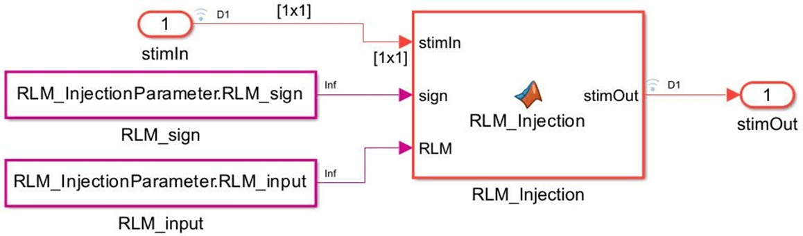
Wire up the input and output ports, along with the two new AMI parameters to the RLM_Injection MATLAB function block. You can also turn logging on for the stimIn and stimOut nodes to visually verify the operation of the RLM Injection.

The RLM pass-through block should look like this:

Refresh Init

At this point you should Refresh Init to ensure all Tx block updates are promoted. You will get a warning that Refresh Init is skipping the newly added RLM_Injection block since it is not a system object. Since RLM is a GetWave only feature, you can ignore this warning.

Analog Channel and Tx/Rx Analog Model Setup

Open the mask for the Analog Channel block and update the following settings:

Confirm the following settings remain the same:

Receiver Model Setup

Open the Rx subsystem. Your canvas should show multiple blocks as follows:

The Rx blocks are summarized below.

Configure Rx Noise Block

To include input referred noise to the receiver, the value needs to be updated for the Node named NoisePSD using the SerDes IBIS-AMI Manager:

Configure Rx CTLE Blocks

To update the CTLE GPZ matrices for 224G, run the attached script genGPZserdesADCCEI224G_MR.m. This script will generate new matrices for the MBZ, CTLE and NF blocks and copy the new matrices to the Simulink Model Workspace. These GPZ matrix values are based on COM values from Table 32-1 in the OIF-CEI-224G-MR specification.

After running the genGPZserdesADCCEI224G_MR.m script, make the following updates to the three CTLE blocks to use the new GPZ matrices:

Open the mask on the MBZ block and update the following variable:

Open the mask on the CTLE block and update the following variable:

Open the mask on the NF block and update the following variable:

Configure Rx SatAmp Block

Along with new GPZ matrices, the genGPZserdesADCCEI224G_MR.m script also generates a new Saturation Amplifier VinVout matrix. To update the matrix:

Open the mask on the SatAmp block and update the following variable:

Configure Rx FFE

In the 112G ADC model used as the starting point for this example, the Rx FFE block used a standard FFE with 3 pre-cursor taps, and 17 post cursor taps. For 224G-MR, the Rx FFE uses 5 pre-cursor taps, 8 post-cursor taps, and 2 sets of 4 floating taps with a maximum span of 50 UI.

The floating taps will be handled in the update to the Rx Init Code Block later in this example.

To update the number of taps and their ranges, in the IBIS-AMI Manager edit the Rx_FFE TapWeights parameter as follows:

Update DFECDR Block

Update the DFECDR block TapWeight.1 values in the IBIS-AMI Manager as follows:

Open the DFECDR block mask and confirm the following settings remain the same:

Then update the following values:

Refresh Init

At this point you should Refresh Init to ensure all Rx block updates are promoted.

Customize Rx Init Code Block

Due to the changes required to support floating taps, the Rx Init code has changed considerably from the ADC IBIS-AMI Model Based on COM that was used as the starting point for this example. The new Rx Init code is included in the adcInitCustomUserCodeCEI224G-MR.m file included with this example.

To modify the custom user code area for Rx Init:

Statistical Adaptation Algorithm Overview

As described in the starting example ADC IBIS-AMI Model Based on COM, the adaptation algorithm for statistical Rx adaptation works as follows:

Run Simulink Model

In the Stimulus block mask set as follows:

In the IBIS-AMI Manager, go to the export tab, and set as follows:

These settings help ensure that the time domain adaptation is able to converge. You can also use a larger number of symbols and ignore bits if investigating correlation of simulation results to measured data.

Update the ADC Quantization

In this example the ADC quantization is also set to 6b by default, and you can change this value as needed, or to observe how the time-domain eye shape is affected by ADC precision. To change the ADC quantization (resolution), update the Resolution (bits) field in the ADC mask.

Generate 224G SerDes IBIS-AMI Models

The final part of this example takes the customized 224G SerDes Simulink model and generates an IBIS-AMI compliant model: including model executables, IBIS and AMI files.

The current IBIS AMI standard does not have native support for ADC-based SerDes. The current standard is written for slicer-based SerDes, which contain a signal node wherein the equalized signal waveform is observed. In a slicer-based SerDes this node exists inside the DFE, right before the decision sampler. A continuous analog waveform is observable at that node, which includes the effect of all the upstream equalizers (such as CTLE) and the equalization due to DFE, as tap weighted and fed back prior decisions. Such a summing node does not exist in an ADC-based SerDes. In a real ADC-based SerDes system the ADC provides a vertical slice though the eye at the sampling instant. To emulate a virtual node, a time-agnostic ADC is used. This ADC quantizes each point in the incoming analog waveform at the simulation time-step rate: i.e. 1/f­­­B/SPS, where SPS is the number of samples per symbol, and fB is the baud-rate. The Rx FFE also processes the input signal as a continuous waveform, rather than as samples. However, the Rx FFE applies single tap values for SPS-simulation time-steps. The DFE is the stock DFE from the SerDes Toolbox and is written for slicer based SerDes. This signal chain allows for the signal integrity simulator to be able to observe a virtual eye in an ADC-based system.

Export IBIS-AMI Models

Open the Export tab in the SerDes IBIS-AMI Manager dialog box.

Utilize IBIS-AMI Models in Simulation

The IBIS-AMI models can now be used in any IBIS-AMI Compliant EDA tool such as Serial Link Designer from Signal Integrity Toolbox.

You can create a project using SI-Link that will automatically launch Serial Link Designer with the IBIS-AMI models included, along with the system variables such as SymbolTime, etc.

You can also launch Serial Link Designer from the MATLAB Command Window with the following command:

>> serialLinkDesigner

Note: For details, please see the documentation page for Serial Link Designer.