Multiple-Edge Response (MER) for AMI Statistical Nonlinear System Analysis
This example demonstrates how to apply AMI equalization to MER characterized impulse-based statistical analysis.
This example will illustrate the complexities of applying AMI equalization to the MER Statistical representation of the system. A traditional IBIS-AMI simulation will process a single impulse response to analyze a system in AMI_Init. In contrast, the MER representation has numerous effective step responses, each needs to be carefully equalized in AMI_Init to obtain meaningful results.
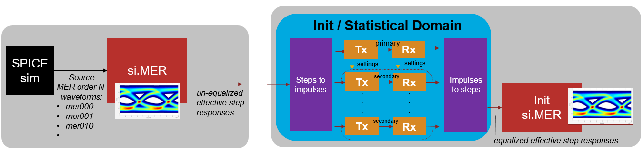
There are two ways of defining the inputs to the si.MER object, one is to generate the source input waveforms as illustrated in the other MER examples and the second is to directly input the effective step responses. This example is all about the effective step responses as illustrated in the analysis overview diagram below. First, create a MER representation with source waveforms as the input and obtain the unequalized effective step responses from the MER object. To apply equalization to these waveforms with AMI models, convert them to impulse responses (which is a standard input to AMI models), process them with the AMI model and then convert them back to step responses with the appropriate polarity (i.e. rising or falling steps). These equalized effective step responses are then used to define the statistical MER object, from which you can get the equalized statistical eye. The nuances and assumptions necessary for this process are outlined in this example.
Generate Nonlinear System MER Effective Step responses
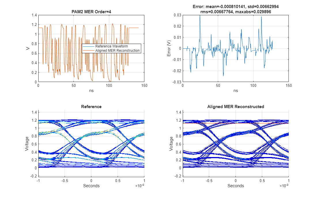
Following the process discussed in Using Multiple-Edge Response (MER) to Represent Nonlinear Systems, extract the MER source waveforms from the Parallel Link Designer Spice simulation results and setup the MER object. A 4th order representation is used to balance the accuracy and complexity of the analysis.
% Define order
Order = 4;

% Define modulation. Must match modulation of SPICE source waveforms
Modulation = 2;

% Define samples per symbol
SamplesPerSymbol = 16;

% Define path to PLD project
ProjectPLD = fullfile(pwd,'MERExamplePLD');

% Define PLD sheet name
sheetname = sprintf('merlin2_order%i',Order);

% Extract PLD data and prepare for AMI simulations.  If the PLD project
% MERExamplePLD doesn't exist yet, then it will be downloaded from the Kit
% repository and simulated.
simData = spice2mer(ProjectPLD, sheetname, Order, SamplesPerSymbol);

% Get source waveforms
SourceWavesPattern = simData.PatternMat;
SourceWaves = simData.PatternWave;
SampleInterval = simData.SampleInterval;
SymbolTime = simData.SymbolTime;

% Create MER representation object
RepMER = si.MER(...
    'Order', Order,...
    'Modulation', Modulation,...
    'SamplesPerSymbol', SamplesPerSymbol,...
    'PlotAxis', 'Seconds',...
    'SymbolTime', SymbolTime,...
    'Specification', 'Wave',...
    'SourceWaves', SourceWaves,...
    'SourceWavesPattern', SourceWavesPattern,...
    'ReferenceWave',simData.ReferenceWave,...
    'ReferenceWavePattern',simData.ReferencePattern);

% Visualize accuracy of MER representation
h1 = figure('IntegerHandle','off');
plotValidation(RepMER)
set(h1,'Units','normalized','Position',[0 0 1 1]);
h2 = figure('IntegerHandle','off');
plotInputs(RepMER)
xlim(min(RepMER.delaySR)*RepMER.SampleInterval*1e9 + SymbolTime*1e9*[-Order,5])
set(h2,'Units','normalized','Position',[ 0 0 1 1]);
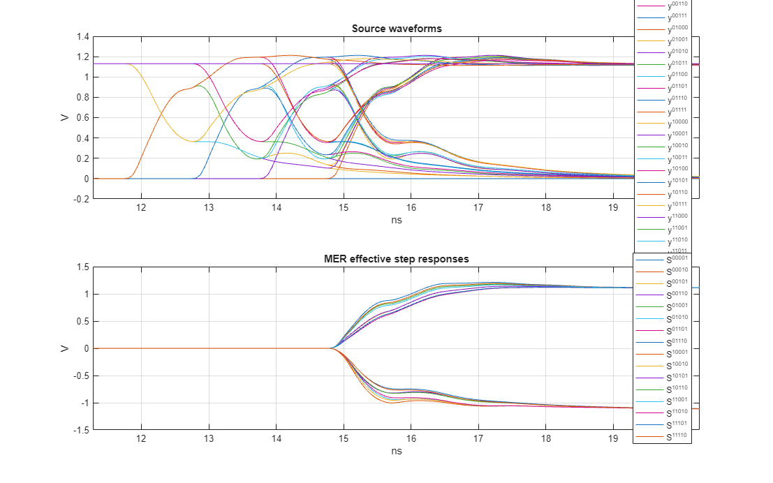
The above figure shows the source waveforms and the resulting effective step responses. See Using Multiple-Edge Response (MER) to Represent Nonlinear Systems for more details on how these are obtained. Calculate the effective impulse responses from the effective step responses. Note that the impulse responses derived from the falling step responses will be negative.
% Get unequalized MER effective step responses of analog channel
effectiveSteps = RepMER.EffectiveSteps;

% Convert effective step responses to impulse responses
effectiveImpulses = step2impulse(effectiveSteps,RepMER.SampleInterval);
Set Up Transmitter AMI System
The serdes.AMI object provides the ability to interact with an AMI model at a very basic level. Whereas modern simulators like Serial Link Designer automatically set up an AMI model, here you can manually control the model and specify inputs via the input string. To do so, provide the ParameterAMI class to assist in creating the input string and to extract data from the output AMI parameter string.
The transmitter AMI model only contains a simple feed-forward equalizer (FFE) with one precursor and three post-cursors. The FFE is not adaptive and can be either off or in fixed mode. Preliminary work found that the transmitter FFE with a 5% post-cursor tap provided a good balance of equalization with the receiver equalization.
% Define the root name
amiRootName = 'simple_serdes';

% Create Tx AMI object
txAMI1 = serdes.AMI;

% Define library name and path
txAMI1.LibraryPath = pwd;
txAMI1.LibraryName = [amiRootName,'_tx_',computer('arch')];

% Set InitOnly to true for Init only analysis
txAMI1.InitOnly = true;

% Define symbol time and sample interval
txAMI1.SymbolTime = SymbolTime;
txAMI1.SampleInterval = SampleInterval;

% Define length of the impulse response
rowSize = size(effectiveImpulses,1);
txAMI1.RowSize = rowSize;

% Define how the model behaves in adapt and fixed mode. This transmitter
% model doesn't adapt, so the adapt mode is the same as fixed.
ModeIndices = 1;
AdaptModeIndex = 1;
FixedModeIndex = 1;
txParameters = ParameterAMI([amiRootName,'_tx.ami'],ModeIndices,AdaptModeIndex,FixedModeIndex);
Summary of mode settings for analysis:
FFE.Mode: Adapt: 1/ fixed, Fixed: 1/ fixed
% Display all parameters
DisplayParameters(txParameters)
All In and InOut AMI Parameters for simple_serdes_tx.ami: 1 FFE.Mode List_Tip (Value:String)| 1:fixed 0:off 2 FFE.TapWeights.m1 3 FFE.TapWeights.p0 4 FFE.TapWeights.p1 5 FFE.TapWeights.p2 6 FFE.TapWeights.p3
% Set transmitter equalization. One pre-cursor and three post-cursor taps.
ffetaps = [0, 0.95, -0.05, 0, 0];
txParameters.SetParameter('FFE.TapWeights.m1',ffetaps(1));
txParameters.SetParameter('FFE.TapWeights.p0',ffetaps(2));
txParameters.SetParameter('FFE.TapWeights.p1',ffetaps(3));
txParameters.SetParameter('FFE.TapWeights.p2',ffetaps(4));
txParameters.SetParameter('FFE.TapWeights.p3',ffetaps(5));

% Set fixed mode behavior and generate transmitter input string.
txInputString = FixedInputString(txParameters);
txAMI1.InputString = txInputString;
disp(txInputString)
(simple_serdes_tx(Modulation "NRZ")(FFE(Mode 1)(TapWeights(-1 0)(0 0.95)(1 -0.05)(2 0)(3 0))))
Set Up Receiver AMI System
The receiver AMI model contains a combined four-tap decision-feedback equalizer (DFE) and clock and data recovery (CDR) block. The receiver model itself was created in SerDes Toolbox's SerDes Designer App and Simulink. The DFE mode can be off, fixed or adapt. In fixed mode, the input DFE tap values are applied for all time, and in adapt mode the input DFE tap values are first estimated from the impulse response in AMI_Init which then initialize the DFE tap values in AMI_GetWave. The GetWave tap values then adapt according to a blind least-mean-squared (LMS) algorithm that attempts to drive the inter-symbol interference (ISI) to zero under the assumption of a totally random data pattern.
The N-tap DFE algorithm to determine the DFE taps in AMI_Init, is based on converting the impulse response to a pulse response and then estimating the location of the sampling clock according to the hula-hoop algorithm. This conceptually drops a one symbol time diameter hoop over the pulse response, with the center of the hoop being the sampling location. From knowing the time location of the clock sampler, the amount of ISI at future samples, 1 to N unit intervals from the clock, is read directly from the pulse response. Therefore, if the pulse response is vertically shifted so that the pulse response is zero at these times, then there would be no ISI to distort the sampled voltage. These hula-hoop and zero-forcing algorithms allow for the application of a complicated behavior to the pulse (and impulse) response in a simple way.
The DFE model in the example model can fully control and specify the DFE tap values when applied to an impulse response, but it relies completely on the hula-hoop algorithm to determine where the DFE taps are applied. This lack of ability to precisely specify the location of the DFE taps will lead to some non-ideal behavior discussed later.
Set up the receiver AMI block and define the settings to place the receiver in fixed mode and adaptive mode.
% Create Rx AMI object
rxAMI1 = serdes.AMI;

% Define library name and path
rxAMI1.LibraryPath = pwd;
rxAMI1.LibraryName = [amiRootName,'_rx_',computer('arch')];
rxAMIfilename = [amiRootName,'_rx.ami'];

% Set InitOnly to true for Init only analysis
rxAMI1.InitOnly = true;

% Define symbol time and sample interval
rxAMI1.SymbolTime = SymbolTime;
rxAMI1.SampleInterval = SampleInterval;

% Define length of the impulse response
rxAMI1.RowSize = rowSize;

% Define how the model behaves in adapt and fixed mode. From the display of
% the parameters, you can identify the indices of the mode, and the
% indices of the List_Tip members. ParameterAMI with only one input
% argument will provide an interactive way of determining the mode indices
% and fixed/adapt settings.
ModeIndices = 1;    % DFECDR.Mode is the first parameter
AdaptModeIndex = 1; % Adapt is the first in the list
FixedModeIndex = 3; % Fixed is the third in the list
rxParameters = ParameterAMI(rxAMIfilename,ModeIndices,AdaptModeIndex,FixedModeIndex);
Summary of mode settings for analysis:
DFECDR.Mode: Adapt: 2/ adapt, Fixed: 1/ fixed
The above summary shares that for the AMI parameter DFECDR.Mode, which the settings used for adapt and fixed mode. The parameter is a "List_Tip" parameter, where the input values of 0 1 2 have aliases of "off" "fixed and "adapt". The summary identifies that for Adapt mode, the parameter will be set to the value of 2 (or "adapt") and for Fixed mode, the parameter will be set to the value of 1 (or "fixed).
% Display all parameters and List_Tip members
DisplayParameters(rxParameters)
All In and InOut AMI Parameters for simple_serdes_rx.ami: 1 DFECDR.Mode List_Tip (Value:String)| 2:adapt 0:off 1:fixed 2 DFECDR.Phase 3 DFECDR.PhaseOffset 4 DFECDR.ReferenceOffset 5 DFECDR.TapWeights.p1 6 DFECDR.TapWeights.p2 7 DFECDR.TapWeights.p3 8 DFECDR.TapWeights.p4
Experiment Setup and AMI Analysis
AMI_Init is based on impulse response processing. Since the system is MER characterized with multiple conditionally-LTI step responses, you can process each of these conditionally-LTI impulse responses with equalization to determine the resulting equalized statistical eye response. It is critical that all responses are equalized with the same equalization settings, otherwise incongruous results will occur. For example, if the impulse responses relating to the rising and falling effective step responses are equalized with a CTLE with different DC gains, then the resulting voltage swing of the equalized impulse responses will be different. When trying to use these imbalanced step responses to reconstruct a waveform, it would be impossible to return to a given terminal voltage after adding the rising and falling step responses together. Therefore, extensive efforts will be made to apply identical equalization settings to all the effective step responses.
Determining the best equalization settings is a very difficult problem. Conduct an experiment which explores three different options for the DFE equalization settings:
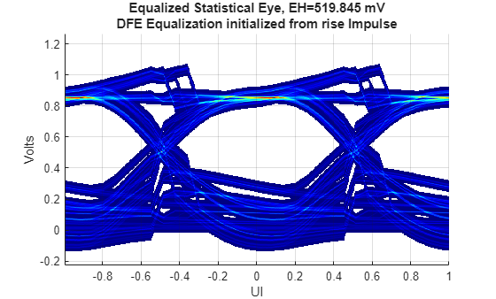
case 1: DFE tap values derived from the rising step response impulse,
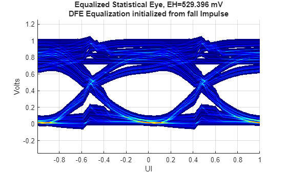
case 2: DFE tap values derived from the falling step response impulse,
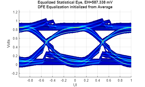
case 3: DFE tap values derived from the average of the above approaches.
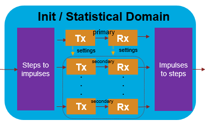
For a NRZ MER order 4, there are 16 effective step responses. For each experimental case, identify the primary impulse response, process it with the DFE in adapt mode and determine the DFE tap values. The DFE block model is then put into fixed mode with these DFE tap values and the remaining secondary impulse responses are processed. The set of impulse responses are then converted to step responses and then input to the MER object to create the equalized statistical eye. An illustration of the processing of the primary and secondary impulse responses is shown below:
% Initialize matrix to save DFE taps
savedDFETaps = zeros(2,4);
ClockIn = -1;
stimulusWave = [];

% Loop over cases
for kk = 1:3

    % Identify primary response index
    if kk==1
        PrimaryResponseIndex = 1;
        label = 'rise Impulse';
    elseif kk==2
        PrimaryResponseIndex = size(effectiveImpulses,2); % 16 for MER order 4
        label = 'fall Impulse';
    else
        PrimaryResponseIndex = 1;
        label = 'Average';
    end
This section of code processes the primary impulse response.
    % Setup primary impulse response
    PrimaryImpulseUnEQ = effectiveImpulses(:,PrimaryResponseIndex);

    % If impulse response is from a falling step response, invert it
    if effectiveSteps(1,PrimaryResponseIndex)>effectiveSteps(end,PrimaryResponseIndex)
        isfall = true;
        %Invert impulse to mimic a rising impulse response
        PrimaryImpulseUnEQ = -PrimaryImpulseUnEQ;
    else
        isfall = false;
    end

    % Determine AMI input string
    if kk < 3
        % Set Rx to adaptive mode
        rxAMI1.InputString = rxParameters.AdaptInputString;
    else % kk==3
        % Set tap weights to average of previous cases
        averagedDFETaps = mean(savedDFETaps,1);
        rxParameters.SetParameter('DFECDR.TapWeights.p1',averagedDFETaps(1));
        rxParameters.SetParameter('DFECDR.TapWeights.p2',averagedDFETaps(2));
        rxParameters.SetParameter('DFECDR.TapWeights.p3',averagedDFETaps(3));
        rxParameters.SetParameter('DFECDR.TapWeights.p4',averagedDFETaps(4));
        % Set rx to fixed mode
        rxAMI1.InputString = rxParameters.FixedInputString;
    end
fprintf('Case %i RX primary input string: %s\n',kk,rxAMI1.InputString);

    % AMI_Init: Primary impulse response analysis
    [~, txImpulsePrimaryOut] = txAMI1(stimulusWave, PrimaryImpulseUnEQ, ClockIn);
    [~, rxImpulsePrimaryOut] = rxAMI1(stimulusWave, txImpulsePrimaryOut, ClockIn);
    % Cleanup and flush results
    txAMI1.release;
    rxAMI1.release;

    if isfall
        % Undo inversion if falling step response
        rxImpulsePrimaryOut = -rxImpulsePrimaryOut;
    end

    % Get output equalization settings
    RxInitOutputParams = rxAMI1.AMIData.InitAMIOutput;
fprintf('Case %i RX output string: %s\n',kk,RxInitOutputParams);

    % Save output DFE tap weight values
    if kk~=3
        structOut = ParameterAMI.ReadAMIString(RxInitOutputParams);
        savedDFETaps(kk,1) = structOut.simple_serdes_rx.DFECDR.TapWeights.p1;
        savedDFETaps(kk,2) = structOut.simple_serdes_rx.DFECDR.TapWeights.p2;
        savedDFETaps(kk,3) = structOut.simple_serdes_rx.DFECDR.TapWeights.p3;
        savedDFETaps(kk,4) = structOut.simple_serdes_rx.DFECDR.TapWeights.p4;
    end
This section of code processes the secondary impulse responses:
    % Set the DFE tap values from the primary impulse analysis
    SetInOut(rxParameters,RxInitOutputParams);

    % Get string for fixed mode analysis
    rxInputString = FixedInputString(rxParameters);
fprintf('Case %i RX secondary input string: %s\n',kk,rxInputString);

    % AMI Analysis with secondary impulse responses (no adaptation)
    rxAMI1.InputString = rxInputString;

    % Loop over remaining impulse responses and process them with the same
    % equalization settings obtained from the primary impulse analysis
    EQeffectiveImpulses = zeros(size(effectiveImpulses));
    EQeffectiveImpulses(:,PrimaryResponseIndex) = rxImpulsePrimaryOut;
    for ii = setdiff(1:size(effectiveImpulses,2),PrimaryResponseIndex)
        InputImpulse = effectiveImpulses(:,ii);

        % Determine if impulse response is from a falling step response
        if effectiveSteps(1,ii)>effectiveSteps(end,ii)
            isfall = true;
            %Invert impulse to mimic a rising impulse response
            InputImpulse = -InputImpulse;
        else
            isfall = false;
        end

        % AMI_Init:
        [~, txImpulseOut] = txAMI1(stimulusWave, InputImpulse, ClockIn);
        [~, rxImpulseOut] = rxAMI1(stimulusWave, txImpulseOut, ClockIn);

        if isfall
            rxImpulseOut = -rxImpulseOut;
        end
        EQeffectiveImpulses(:,ii) = rxImpulseOut;

        % Cleanup and flush results
        txAMI1.release;
        rxAMI1.release;
    end
Once all impulse responses are processed with the same equalization settings, convert them to step responses and define a MER object with them. This allows for the creation of a statistical equalized eye diagram, where you can quantify the system performance with eye metrics.
    % impulse to step responses, create equalized MER response
    EQeffectiveSteps = impulse2step(EQeffectiveImpulses,SampleInterval);

    % Determine symbol voltages of equalized signal
    SymbolVoltageEstimate = [0,mean(abs(EQeffectiveSteps(end,:)))+std(abs(EQeffectiveSteps(end,:)))];

    % Generate MER statistical eye diagram
    EQInitMER = si.MER('Order',RepMER.Order,...
        'Modulation',RepMER.Modulation,...
        'SymbolTime',RepMER.SymbolTime,...
        'SamplesPerSymbol',RepMER.SamplesPerSymbol,...
        'Specification','Step',...
        'SourceEffectiveSteps',EQeffectiveSteps,...
        'SourceEffectiveStepsPattern',RepMER.EffectiveStepsPattern,...
        'SourceSymbolVoltage',SymbolVoltageEstimate);

figure('IntegerHandle','off');
plotStateye(EQInitMER)
    title(sprintf('Equalized Statistical Eye, EH=%g mV\nDFE Equalization initialized from %s',...
        EQInitMER.StatEyeInfo.EyeObj.eyeHeight*1e3,label))
end
Case 1 RX primary input string: (simple_serdes_rx(Modulation "NRZ")(DFECDR(ReferenceOffset 0)(PhaseOffset 0)(Mode 2)(TapWeights(1 0)(2 0)(3 0)(4 0))))
Case 1 RX output string: (simple_serdes_rx(DFECDR(Phase 16.7228)(TapWeights(1 -0.242675)(2 0.03353)(3 0.044843)(4 0.010119))))
Case 1 RX secondary input string: (simple_serdes_rx(Modulation "NRZ")(DFECDR(ReferenceOffset 0)(PhaseOffset 0)(Mode 1)(TapWeights(1 -0.24268)(2 0.03353)(3 0.044843)(4 0.010119))))
Case 2 RX primary input string: (simple_serdes_rx(Modulation "NRZ")(DFECDR(ReferenceOffset 0)(PhaseOffset 0)(Mode 2)(TapWeights(1 -0.24268)(2 0.03353)(3 0.044843)(4 0.010119))))
Case 3 RX primary input string: (simple_serdes_rx(Modulation "NRZ")(DFECDR(ReferenceOffset 0)(PhaseOffset 0)(Mode 1)(TapWeights(1 -0.17403)(2 -0.033222)(3 -0.000919)(4 -0.005359))))
Case 2 RX output string: (simple_serdes_rx(DFECDR(Phase 16.7086)(TapWeights(1 -0.10539)(2 -0.099974)(3 -0.046681)(4 -0.020837))))
Case 2 RX secondary input string: (simple_serdes_rx(Modulation "NRZ")(DFECDR(ReferenceOffset 0)(PhaseOffset 0)(Mode 1)(TapWeights(1 -0.10539)(2 -0.099974)(3 -0.046681)(4 -0.020837))))
Case 3 RX output string: (simple_serdes_rx(DFECDR(Phase 16.7228)(TapWeights(1 -0.17403)(2 -0.033222)(3 -0.000919)(4 -0.005359))))
Case 3 RX secondary input string: (simple_serdes_rx(Modulation "NRZ")(DFECDR(ReferenceOffset 0)(PhaseOffset 0)(Mode 1)(TapWeights(1 -0.17403)(2 -0.033222)(3 -0.000919)(4 -0.005359))))
Analyzing Experimental Results
When the DFE tap values are derived from the rising step response impulse, the upper symbol voltage of the eye diagram is well equalized, but the lower symbol voltage is poorly controlled. And when the DFE tap values are derived from the falling step response impulse, the lower symbol voltage of the eye diagram is well equalized, but the upper symbol voltage is dispersed. When the average of the first two case DFE taps is used, neither upper nor lower eye voltages are tight, but the overall effect is a 60 to 70 mV improvement in eye height. Determining the optimal DFE tap values for this type of nonlinear system would be an interesting point of future research.
A tell-tale sign of a DFE is the abrupt voltage jump at the edges of the eye or symbol boundary. What is unique about these eye diagrams is that there are a few different time locations for the voltage jump. While this is expected in a time domain eye, in statistical, the voltage jumps should all be aligned. This is a limitation of the DFE model's inability to exactly replicate the primary impulse response equalization settings for the secondary impulse response equalization. The DFE hula-hoop CDR algorithm relies on the input impulse response to determine the clock location, but due to the variability inherent in the effective step impulse responses, different clock locations were used when applying the DFE taps. Creating AMI models that can better handle this behavior is a point of future development. Likely, this irregularity of CDR location pessimistically reduced eye height by a small amount.
Comparing the statistical eyes in this example to the eye diagrams in Multiple-Edge Response (MER) for AMI Fast Time-Domain Nonlinear System Simulation, observe the following:
The reported statistical eye heights are smaller by about 30 to 40 mV. This is due to the nature of statistical eyes and their deep pattern reach of ISI. A time domain eye would need to run for billions of symbols to reach the BER depth of statistical eyes. Further, the statistical DFE clock location issue pessimistically reduced the eye height by some unknown amount.
The eye height difference between the average case and the cases derived from the rising/falling steps is roughly 60 to 70 mV for both the time domain and the statistical eyes. This curious consistency will need to be explored by using other interconnect channels and data rates to determine if this consistency is significant or not.
Summary
This example illustrates a proposed solution to applying equalization to MER effective step responses and the creation of AMI equalized MER statistical eye diagrams. Much care is taken to apply nearly identical equalization settings to all of the effective step responses.
Explore further by
Choosing other impulse responses from the set, other than 1 and 16, to derive the DFE taps from.
Applying the flow to your own AMI models.
Ideas for future research:
Use the SerDes Toolbox to create a DFE block for AMI models which allows for specification of the DFE clock location.
Create an AMI model which can process all the effective step responses simultaneously. Perhaps, new methods of determining optimal DFE taps can be found.
Propose an extension to the IBIS-AMI standard such that AMI_Init can accept all of the effective step responses directly, determine the optimal equalization settings and apply the equalization to the effective step responses.
Determine how to include crosstalk into the MER analysis. Since crosstalk is proportional to the edge rate, the crosstalk may need MER treatment but perhaps not to the same degree as the primary signal.
Apply methodology to optical systems which also suffer from rising/falling edge time mismatch.