Radar Pulse Compression
This example shows the effects of pulse compression, where a transmitted pulse is modulated and correlated with the received signal. Pulse compression is used in radar and sonar systems to improve signal-to-noise ratio (SNR) and range resolution by shortening the duration of echoes.
Time Domain Cross-Correlation
Rectangular Chirp
First, visualize pulse compression with a rectangular pulse. Create a one-second long pulse with a frequency f0 of 10 Hz and a sample rate fs of 1 kHz.
fs = 1e3;
tmax = 15;
tt = 0:1/fs:tmax-1/fs;
f0 = 10;
T = 1;
t = 0:1/fs:T-1/fs;
pls = cos(2*pi*f0*t);
Create the received signal starting at 5 seconds based off the original pulse without any noise. The signal represents increasingly distant targets whose reflected signals are separated by 2 seconds. The reflectivity term ref determines what fraction of the transmitted power the received pulse has. The attenuation factor att dictates how much the signal strength decreases over time.
t0 = 5;
dt = 2*T;
lgs = t0:dt:tmax;
att = 1.1;
ref = 0.2;
rpls = pulstran(tt,[lgs;ref*att.^-(lgs-t0)]',pls,fs);
Add Gaussian white noise. Specify an SNR of 15 dB.
SNR = 15;
r = randn(size(tt))*std(pls)/db2mag(SNR);
rplsnoise = r+rpls;
Cross-correlate the received signal with the transmitted pulse and plot the processed signal. The transmitted pulse, the received pulse without noise, and the noisy received signal are plotted in the upper graph for convenience.
[m,lg] = xcorr(rplsnoise,pls);
m = m(lg>=0);
tm = lg(lg>=0)/fs;

subplot(2,1,1)
plot(tt,rplsnoise,t,pls,tt,rpls)
xticks(lgs)
legend('Noisy Received','Initial Pulse','Noiseless Received')
title('Transmitted/Received Signals')
ylabel('Magnitude (L.U.)')

subplot(2,1,2)
plot(tm,abs(m))
xticks(lgs)
title('Matched Filter Output')
xlabel('Time (s)')
ylabel('Magnitude (L.U.)')
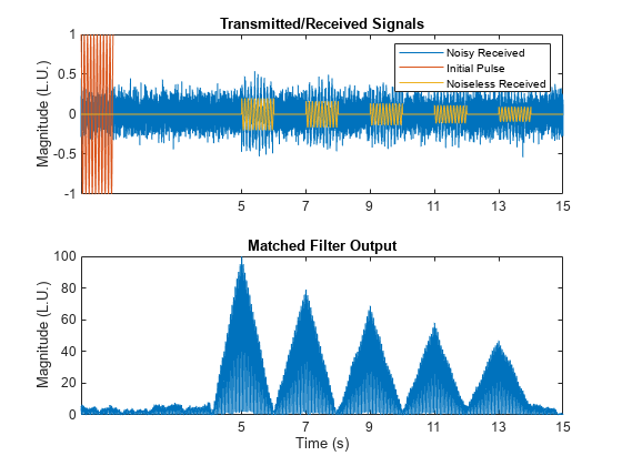
If these were echoes from multiple targets, it would be possible to get a general idea of the targets' locations because the echoes are spread far enough apart. However, if the targets are closer together, their responses mix.
dt = 1.5*T;
lgs = t0:dt:tmax;
rpls = pulstran(tt,[lgs;ref*att.^-(lgs-t0)]',pls,fs);
rplsnoise = r + rpls;
[m,lg] = xcorr(rplsnoise,pls);
m = m(lg>=0);
tm = lg(lg>=0)/fs;

subplot(2,1,1)
plot(tt,r,t,pls,tt,rpls)
xticks(lgs)
legend('Noisy Received','Initial Pulse','Noiseless Received')
title('Transmitted/Received Signals')
ylabel('Magnitude (L.U.)')

subplot(2,1,2)
plot(tm,abs(m))
xticks(lgs)
title('Matched Filter Output')
xlabel('Time (s)')
ylabel('Magnitude (L.U.)')
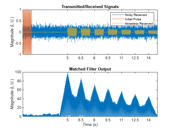
To improve range resolution, or the ability to detect closely-spaced targets, use a linear frequency modulated pulse for cross-correlation.
Linear Frequency Modulated (FM) Chirp
Complete the same procedure but with a complex chirp with a frequency that starts at 0 Hz and linearly increases to 10 Hz. Real-world radar systems often use complex-valued linear FM signals to improve range resolution because the matched filter response is larger and narrower. Since there is an imaginary component to the chirp and matched filter, all plots must be made using the real part of the waveform.
pls = chirp(t,0,T,f0,'complex');
rpls = pulstran(tt,[lgs;ref*att.^-(lgs-t0)]',pls,fs);
r = randn(size(tt))*std(pls)/db2mag(SNR);
rplsnoise = r + rpls;

[m,lg] = xcorr(rplsnoise,pls);
m = m(lg>=0);
tm = lg(lg>=0)/fs;

subplot(2,1,1)
plot(tt,real(r),t,real(pls),tt,real(rpls))
xticks(lgs)
legend('Noisy Received','Initial Pulse','Noiseless Received')
title('Transmitted/Received Signals')
ylabel('Magnitude (L.U.)')

subplot(2,1,2)
plot(tm,abs(m))
xticks(lgs)
title('Matched Filter Output')
xlabel('Time (s)')
ylabel('Magnitude (L.U.)')
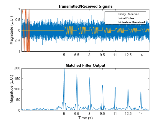
The cross-correlation with a linear FM chirp provides much finer resolution for target noise despite the target echoes being closer together. The sidelobes of the echoes are also greatly reduced compared to the rectangular chirp, allowing for more accurate target detection.
Frequency-Domain Convolution
While cross-correlation does improve the range resolution, the algorithm lends itself better to analog hardware implementation. More commonly, radar systems employ a similar process in the digital domain called matched filtering, where the received signal is convolved with a time-reversed version of the transmitted pulse. Matched filtering is often done in the frequency domain because convolution in the time domain is equivalent to multiplication in the frequency domain, making the process faster. Because the initial pulse is time-reversed, the filtered output is delayed by the pulse width T, which is 1 second.
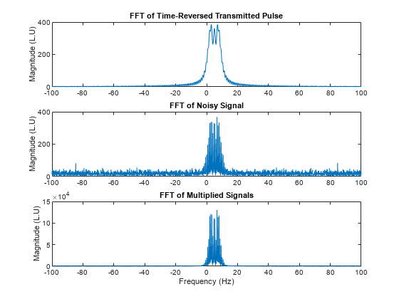
To show this, time-reverse the original linear FM pulse and pad the pulse with zeros to make the pulse and transmitted waveform the same length. Calculate and plot the Fourier transform of the complex conjugate of the time-reversed pulse and the noisy signal. Multiply the two pulses in the frequency domain and plot the product
pls_rev = [fliplr(pls) zeros(1, length(r) - length(pls))];
PLS = fft(conj(pls_rev));
R = fft(rplsnoise);
fft_conv = PLS.*R;
faxis = linspace(-fs/2,fs/2,length(PLS));

clf
subplot(3,1,1)
plot(faxis,abs(fftshift(PLS)))
title('FFT of Time-Reversed Transmitted Pulse')
xlim([-100 100])
ylabel('Magnitude (L.U)')

subplot(3,1,2)
plot(faxis,abs(fftshift(R)))
title('FFT of Noisy Signal')
xlim([-100 100])
ylabel('Magnitude (L.U)')

subplot(3,1,3)
plot(faxis,abs(fftshift(fft_conv)))
title("FFT of Multiplied Signals")
xlabel('Frequency (Hz)')
xlim([-100 100])
ylabel('Magnitude (L.U)')
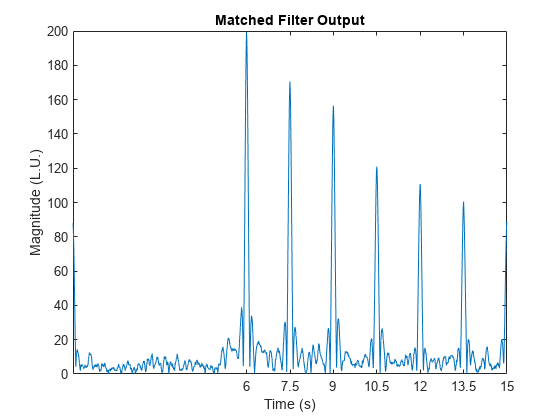
Convert the resulting signal back to the time domain and plot it.
pls_prod = ifft(fft_conv);

clf
plot((0:length(pls_prod)-1)/fs,abs(pls_prod))
xticks(lgs+T)
xlabel('Time (s)')
ylabel('Magnitude (L.U.)')
title('Matched Filter Output')
Sidelobe Reduction Using Windows
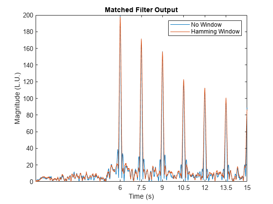
To smooth out the sidelobes after matched filtering, apply a window to the transmitted pulse before time-reversing. The steps in the previous section were shown to better visualize the process of matched filtering in the frequency domain. The function fftfilt can quickly apply matched filtering to a function.
n = fftfilt(fliplr(conj(pls)),rplsnoise);
n_win = fftfilt(fliplr(conj(pls).*taylorwin(length(pls), 30)'),rplsnoise);

clf
plot(tt,abs(n),tt,abs(n_win))
xticks(lgs+T)
xlabel('Time (s)')
ylabel('Magnitude (L.U.)')
legend('No Window', 'Hamming Window')
title('Matched Filter Output')
Doppler Shifted Targets
When a radar pulse is reflected off a stationary target, the pulse is unmodulated and thus has a large response when the transmitted waveform is used for matched filtering. However, moving targets reflect Doppler shifted pulses, making the response from matched filtering less strong. One solution to this is to use a bank of matched filters with Doppler shifted waveforms, which can be used to determine the Doppler shift of the reflected pulse. The radar system can estimate the target velocity, as the Doppler shift is proportional to the velocity.
To show Doppler processing using a bank of matched filters, create a response that is Doppler shifted by 5 Hz.
pls = chirp(t,0,T,f0, 'complex');
shift = 5;
pls_shift = chirp(t,shift,T,f0+shift,'complex');
rpls_shift = pulstran(tt,[lgs;ref*att.^-(lgs-t0)]',pls_shift,fs);
r = (randn(size(tt)) + 1j*randn(size(tt)))*std(pls)/db2mag(SNR);
rplsnoise_shift = r + rpls_shift;
Create a bank of Doppler shifted pulses and observe the difference in response for each matched filter.
filters = [];
for foffset = 0:4:10
    filters = [filters; chirp(t,0+foffset,T,f0+foffset,'complex')];
end
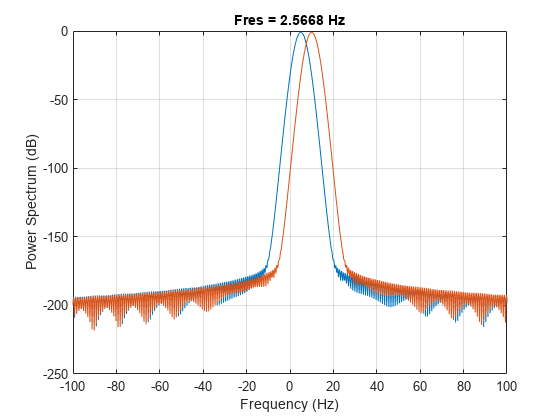
Plotting the frequency domain of the original pulse and the new pulse shows that the new pulse is offset by 5 Hz.
clf
pspectrum([pls; pls_shift].',fs)
xlim([-100 100])
Apply each matched filter to the frequency-shifted pulse and plot the output.
matched_pls = fftfilt(fliplr(conj(pls_shift)),rplsnoise_shift);
filt_bank_pulses = fftfilt(fliplr(filters)',rplsnoise_shift);

clf
subplot(2,1,1)
plot(tt,abs(matched_pls),'Color',[0.6350, 0.0780, 0.1840])
title('Matched Filter (5 Hz)')
ylabel('Magnitude (L.U.)')
xticks(lgs+T)
subplot(2,1,2)
plot(tt, abs(filt_bank_pulses))
legend("0 Hz", "4 Hz", "8 Hz")
title('Matched Filter Bank')
xlabel('Time (s)')
ylabel('Magnitude (L.U.)')
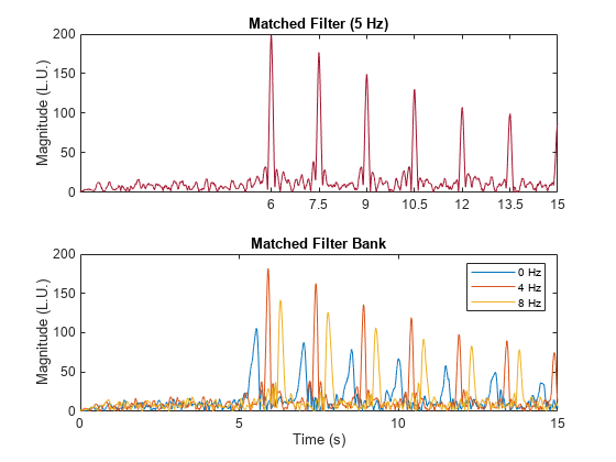
The plot with all three outputs shows that the matched filter shifted by 4 Hz has the greatest response, so the radar system would approximate the Doppler shift to be around 4 Hz. Using more Doppler filters with smaller frequency-shift intervals can help improve the Doppler resolution.
This method of Doppler processing is often not used due to the slower nature of applying many filters. Most signal processing on radar returns is done with a data cube, where the three dimensions are the fast time samples (range response within a pulse), the number of array elements, and the slow time samples (number of pulses). After the system determines the range of the object, a Fourier transform is done across the slow time dimension to determine the Doppler of the target. For this setup, the data cube method would not be ideal for Doppler processing since the system transmits only one pulse. The data cube method works best when you have numerous pulses, which is why many radar systems use a pulse train, or a series of pulses, rather than a single pulse for range-Doppler processing.