PredictionConfidenceInterval
Object containing confidence interval results for model predictions
Description
The PredictionConfidenceInterval object contains confidence
interval results for model predictions (that is, simulation results based on estimated
parameters).
Creation
Create a prediction confidence interval object using sbiopredictionci.
Properties
This property is read-only.
Names of model responses in the parameter fit, specified as a cell array of character vectors. Each cell contains the name of a response.
Example: {'Central.Drug_Central' }
{'Peripheral.Drug_Peripheral'}
This property is read-only.
Confidence interval estimation status, specified as one of the following categorical values:
success– The proper confidence intervals are found. That is, no model prediction is constrained by the parameter bounds defined in the original fit.constrained– The confidence intervals are found, but the confidence interval for the model response is constrained by a parameter bound defined in the original fit.not estimable– No confidence intervals are found.estimable– The proper confidence intervals are found, but other model predictions have an estimation status of eitherconstrainedornot estimable. For the bootstrap confidence interval, the status is always set toestimable.
For details, see Gaussian Confidence Interval Calculation for Model Predictions and Bootstrap Confidence Interval Calculation.
Example: success
This property is read-only.
Confidence interval type, specified as 'gaussian' or
'bootstrap'.
Example: 'bootstrap'
This property is read-only.
Confidence level, (1-Alpha) * 100%, specified as a
positive scalar between 0 and 1.
Example: 0.01
This property is read-only.
Original group names from the data used for fitting the model, specified as a cell array of character vectors. Each cell contains the name of a group.
Example: {'1'}{'2'}{'3'}
This property is read-only.
Confidence interval results, specified as a table. The table contains the following columns.
| Column Name | Description |
|---|---|
| Group | Group name |
| Response | Model response name |
| Time | Simulation time |
| Estimate | Estimated response value |
| ConfidenceInterval | Confidence interval values |
This property is read-only.
Exit flags returned during the calculation of bootstrap
confidence intervals only, specified as a vector of integers. Each integer
is an exit flag returned by the estimation function (except
nlinfit) used to fit parameters during
bootstrapping. The same estimation function used in the original fit is used
for bootstrapping.
Each flag indicates the success or failure status of the fitting performed to create a bootstrap sample. Refer to the reference page of the corresponding estimation function for the meaning of the exit flag.
If the estimation function does not return an exit flag,
ExitFlags is set to []. For the
gaussian confidence intervals,
ExitFlags is not supported and is always set to
[].
Object Functions
plot | Plot confidence interval results for model predictions |
Examples
Load Data
Load the sample data to fit. The data is stored as a table with variables ID , Time , CentralConc , and PeripheralConc. This synthetic data represents the time course of plasma concentrations measured at eight different time points for both central and peripheral compartments after an infusion dose for three individuals.
load data10_32R.mat
gData = groupedData(data);
gData.Properties.VariableUnits = {'','hour','milligram/liter','milligram/liter'};
sbiotrellis(gData,'ID','Time',{'CentralConc','PeripheralConc'},'Marker','+',...
            'LineStyle','none');

Create Model
Create a two-compartment model.
pkmd                 = PKModelDesign;
pkc1                 = addCompartment(pkmd,'Central');
pkc1.DosingType      = 'Infusion';
pkc1.EliminationType = 'linear-clearance';
pkc1.HasResponseVariable = true;
pkc2                 = addCompartment(pkmd,'Peripheral');
model                = construct(pkmd);
configset            = getconfigset(model);
configset.CompileOptions.UnitConversion = true;
Define Dosing
Define the infusion dose.
dose             = sbiodose('dose','TargetName','Drug_Central');
dose.StartTime   = 0;
dose.Amount      = 100;
dose.Rate        = 50;
dose.AmountUnits = 'milligram';
dose.TimeUnits   = 'hour';
dose.RateUnits   = 'milligram/hour';
Define Parameters
Define the parameters to estimate. Set the parameter bounds for each parameter. In addition to these explicit bounds, the parameter transformations (such as log, logit, or probit) impose implicit bounds.
responseMap = {'Drug_Central = CentralConc','Drug_Peripheral = PeripheralConc'};
paramsToEstimate   = {'log(Central)','log(Peripheral)','Q12','Cl_Central'};
estimatedParam     = estimatedInfo(paramsToEstimate,...
                                   'InitialValue',[1 1 1 1],...
                                   'Bounds',[0.1 3;0.1 10;0 10;0.1 2]);
Fit Model
Perform an unpooled fit, that is, one set of estimated parameters for each patient.
unpooledFit = sbiofit(model,gData,responseMap,estimatedParam,dose,'Pooled',false);
Perform a pooled fit, that is, one set of estimated parameters for all patients.
pooledFit = sbiofit(model,gData,responseMap,estimatedParam,dose,'Pooled',true);
Compute Confidence Intervals for Estimated Parameters
Compute 95% confidence intervals for each estimated parameter in the unpooled fit.
ciParamUnpooled = sbioparameterci(unpooledFit);
Display Results
Display the confidence intervals in a table format. For details about the meaning of each estimation status, see Parameter Confidence Interval Estimation Status.
ci2table(ciParamUnpooled)
ans =

  12×7 table

    Group         Name         Estimate    ConfidenceInterval      Type      Alpha      Status
    _____    ______________    ________    __________________    ________    _____    ___________

      1      {'Central'   }      1.422      1.1533     1.6906    Gaussian    0.05     estimable
      1      {'Peripheral'}     1.5629     0.83143     2.3551    Gaussian    0.05     constrained
      1      {'Q12'       }    0.47159     0.20093    0.80247    Gaussian    0.05     constrained
      1      {'Cl_Central'}    0.52898     0.44842    0.60955    Gaussian    0.05     estimable
      2      {'Central'   }     1.8322      1.7893     1.8751    Gaussian    0.05     success
      2      {'Peripheral'}     5.3368      3.9133     6.7602    Gaussian    0.05     success
      2      {'Q12'       }    0.27641      0.2093    0.34351    Gaussian    0.05     success
      2      {'Cl_Central'}    0.86034     0.80313    0.91755    Gaussian    0.05     success
      3      {'Central'   }     1.6657      1.5818     1.7497    Gaussian    0.05     success
      3      {'Peripheral'}     5.5632      4.7557     6.3708    Gaussian    0.05     success
      3      {'Q12'       }    0.78361     0.65581    0.91142    Gaussian    0.05     success
      3      {'Cl_Central'}     1.0233     0.96375     1.0828    Gaussian    0.05     success
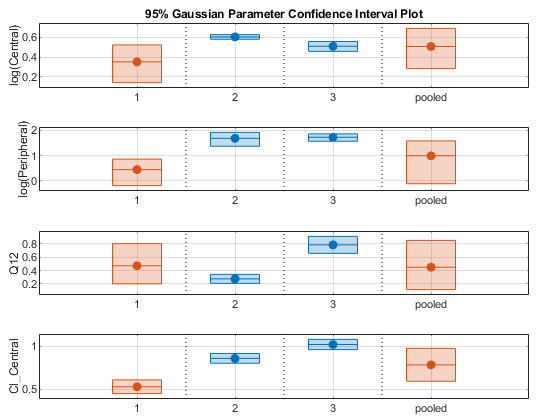
Plot the confidence intervals. If the estimation status of a confidence interval is success, it is plotted in blue (the first default color). Otherwise, it is plotted in red (the second default color), which indicates that further investigation into the fitted parameters may be required. If the confidence interval is not estimable, then the function plots a red line with a centered cross. If there are any transformed parameters with estimated values 0 (for the log transform) and 1 or 0 (for the probit or logit transform), then no confidence intervals are plotted for those parameter estimates. To see the color order, type get(groot,'defaultAxesColorOrder').
Groups are displayed from left to right in the same order that they appear in the GroupNames property of the object, which is used to label the x-axis. The y-labels are the transformed parameter names.
plot(ciParamUnpooled)

Compute the confidence intervals for the pooled fit.
ciParamPooled = sbioparameterci(pooledFit);
Display the confidence intervals.
ci2table(ciParamPooled)
ans =

  4×7 table

    Group          Name         Estimate    ConfidenceInterval      Type      Alpha      Status
    ______    ______________    ________    __________________    ________    _____    ___________

    pooled    {'Central'   }     1.6626      1.3287     1.9965    Gaussian    0.05     estimable
    pooled    {'Peripheral'}      2.687     0.89848     4.8323    Gaussian    0.05     constrained
    pooled    {'Q12'       }    0.44956     0.11445    0.85152    Gaussian    0.05     constrained
    pooled    {'Cl_Central'}    0.78493     0.59222    0.97764    Gaussian    0.05     estimable
Plot the confidence intervals. The group name is labeled as "pooled" to indicate such fit.
plot(ciParamPooled)

Plot all the confidence interval results together. By default, the confidence interval for each parameter estimate is plotted on a separate axes. Vertical lines group confidence intervals of parameter estimates that were computed in a common fit.
ciAll = [ciParamUnpooled;ciParamPooled];
plot(ciAll)

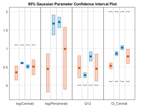
You can also plot all confidence intervals in one axes grouped by parameter estimates using the 'Grouped' layout.
plot(ciAll,'Layout','Grouped')

In this layout, you can point to the center marker of each confidence interval to see the group name. Each estimated parameter is separated by a vertical black line. Vertical dotted lines group confidence intervals of parameter estimates that were computed in a common fit. Parameter bounds defined in the original fit are marked by square brackets. Note the different scales on the y-axis due to parameter transformations. For instance, the y-axis of Q12 is in the linear scale, but that of Central is in the log scale due to its log transform.
Compute Confidence Intervals for Model Predictions
Calculate 95% confidence intervals for the model predictions, that is, simulation results using the estimated parameters.
% For the pooled fit
ciPredPooled = sbiopredictionci(pooledFit);
% For the unpooled fit
ciPredUnpooled = sbiopredictionci(unpooledFit);
Plot Confidence Intervals for Model Predictions
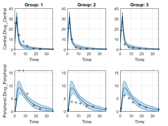
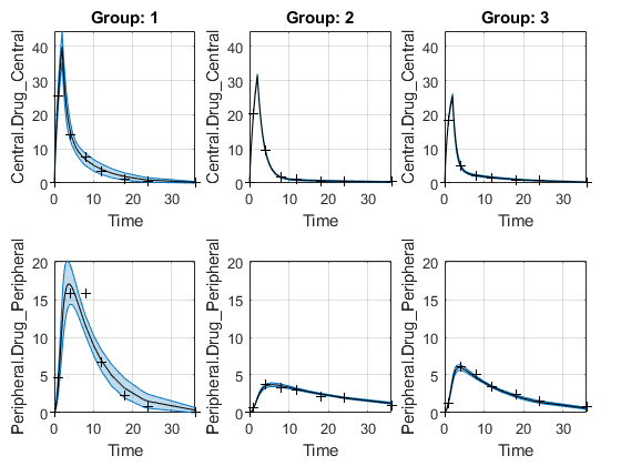
The confidence interval for each group is plotted in a separate column, and each response is plotted in a separate row. Confidence intervals limited by the bounds are plotted in red. Confidence intervals not limited by the bounds are plotted in blue.
plot(ciPredPooled)

plot(ciPredUnpooled)

Version History
Introduced in R2017b
MATLAB Command
You clicked a link that corresponds to this MATLAB command:
Run the command by entering it in the MATLAB Command Window. Web browsers do not support MATLAB commands.
选择网站
选择网站以获取翻译的可用内容,以及查看当地活动和优惠。根据您的位置,我们建议您选择:。
您也可以从以下列表中选择网站:
如何获得最佳网站性能
选择中国网站(中文或英文)以获得最佳网站性能。其他 MathWorks 国家/地区网站并未针对您所在位置的访问进行优化。
美洲
- América Latina (Español)
- Canada (English)
- United States (English)
欧洲
- Belgium (English)
- Denmark (English)
- Deutschland (Deutsch)
- España (Español)
- Finland (English)
- France (Français)
- Ireland (English)
- Italia (Italiano)
- Luxembourg (English)
- Netherlands (English)
- Norway (English)
- Österreich (Deutsch)
- Portugal (English)
- Sweden (English)
- Switzerland
- United Kingdom (English)