sbiopredictionci

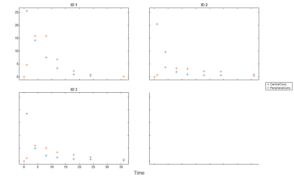
Load Data

Load the sample data to fit. The data is stored as a table with variables ID , Time , CentralConc , and PeripheralConc. This synthetic data represents the time course of plasma concentrations measured at eight different time points for both central and peripheral compartments after an infusion dose for three individuals.

load data10_32R.mat
gData = groupedData(data);
gData.Properties.VariableUnits = {'','hour','milligram/liter','milligram/liter'};
sbiotrellis(gData,'ID','Time',{'CentralConc','PeripheralConc'},'Marker','+',...
            'LineStyle','none');

Create Model

Create a two-compartment model.

pkmd                 = PKModelDesign;
pkc1                 = addCompartment(pkmd,'Central');
pkc1.DosingType      = 'Infusion';
pkc1.EliminationType = 'linear-clearance';
pkc1.HasResponseVariable = true;
pkc2                 = addCompartment(pkmd,'Peripheral');
model                = construct(pkmd);
configset            = getconfigset(model);
configset.CompileOptions.UnitConversion = true;

Define Dosing

Define the infusion dose.

dose             = sbiodose('dose','TargetName','Drug_Central');
dose.StartTime   = 0;
dose.Amount      = 100;
dose.Rate        = 50;
dose.AmountUnits = 'milligram';
dose.TimeUnits   = 'hour';
dose.RateUnits   = 'milligram/hour';

Define Parameters

Define the parameters to estimate. Set the parameter bounds for each parameter. In addition to these explicit bounds, the parameter transformations (such as log, logit, or probit) impose implicit bounds.

responseMap = {'Drug_Central = CentralConc','Drug_Peripheral = PeripheralConc'};
paramsToEstimate   = {'log(Central)','log(Peripheral)','Q12','Cl_Central'};
estimatedParam     = estimatedInfo(paramsToEstimate,...
                                   'InitialValue',[1 1 1 1],...
                                   'Bounds',[0.1 3;0.1 10;0 10;0.1 2]);

Fit Model

Perform an unpooled fit, that is, one set of estimated parameters for each patient.

unpooledFit = sbiofit(model,gData,responseMap,estimatedParam,dose,'Pooled',false);

Perform a pooled fit, that is, one set of estimated parameters for all patients.

pooledFit = sbiofit(model,gData,responseMap,estimatedParam,dose,'Pooled',true);

Compute Confidence Intervals for Estimated Parameters

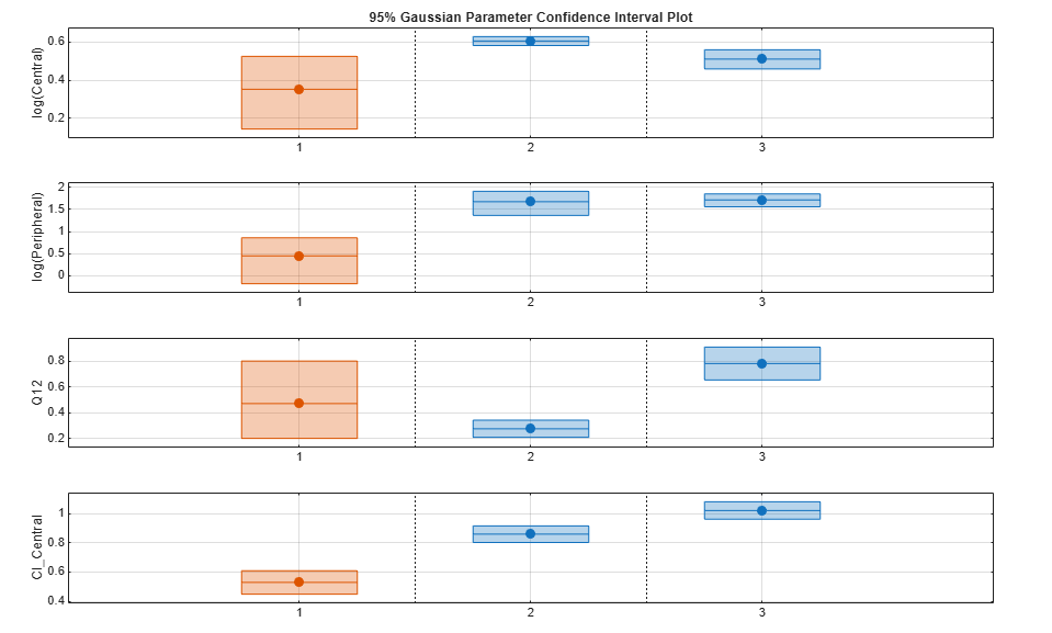
Compute 95% confidence intervals for each estimated parameter in the unpooled fit.

ciParamUnpooled = sbioparameterci(unpooledFit);

Display Results

Display the confidence intervals in a table format. For details about the meaning of each estimation status, see Parameter Confidence Interval Estimation Status.

ci2table(ciParamUnpooled)

ans =

  12x7 table

    Group         Name         Estimate    ConfidenceInterval      Type      Alpha      Status   
    _____    ______________    ________    __________________    ________    _____    ___________

      1      {'Central'   }      1.422      1.1533     1.6906    Gaussian    0.05     estimable  
      1      {'Peripheral'}     1.5629     0.83143     2.3551    Gaussian    0.05     constrained
      1      {'Q12'       }    0.47159     0.20093    0.80247    Gaussian    0.05     constrained
      1      {'Cl_Central'}    0.52898     0.44842    0.60955    Gaussian    0.05     estimable  
      2      {'Central'   }     1.8322      1.7893     1.8751    Gaussian    0.05     success    
      2      {'Peripheral'}     5.3368      3.9133     6.7602    Gaussian    0.05     success    
      2      {'Q12'       }    0.27641      0.2093    0.34351    Gaussian    0.05     success    
      2      {'Cl_Central'}    0.86034     0.80313    0.91755    Gaussian    0.05     success    
      3      {'Central'   }     1.6657      1.5818     1.7497    Gaussian    0.05     success    
      3      {'Peripheral'}     5.5632      4.7557     6.3708    Gaussian    0.05     success    
      3      {'Q12'       }    0.78361     0.65581    0.91142    Gaussian    0.05     success    
      3      {'Cl_Central'}     1.0233     0.96375     1.0828    Gaussian    0.05     success    

Plot the confidence intervals. If the estimation status of a confidence interval is success, it is plotted in blue (the first default color). Otherwise, it is plotted in red (the second default color), which indicates that further investigation into the fitted parameters may be required. If the confidence interval is not estimable, then the function plots a red line with a centered cross. If there are any transformed parameters with estimated values 0 (for the log transform) and 1 or 0 (for the probit or logit transform), then no confidence intervals are plotted for those parameter estimates. To see the color order, type get(groot,'defaultAxesColorOrder').

Groups are displayed from left to right in the same order that they appear in the GroupNames property of the object, which is used to label the x-axis. The y-labels are the transformed parameter names.

plot(ciParamUnpooled)

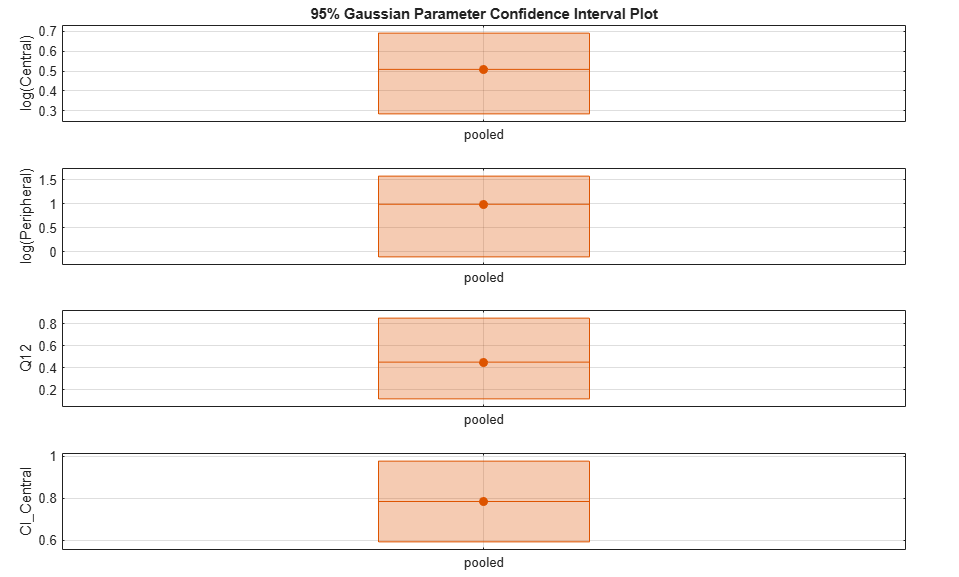
Compute the confidence intervals for the pooled fit.

ciParamPooled = sbioparameterci(pooledFit);

Display the confidence intervals.

ci2table(ciParamPooled)

ans =

  4x7 table

    Group          Name         Estimate    ConfidenceInterval      Type      Alpha      Status   
    ______    ______________    ________    __________________    ________    _____    ___________

    pooled    {'Central'   }     1.6626      1.3287     1.9965    Gaussian    0.05     estimable  
    pooled    {'Peripheral'}      2.687     0.89848     4.8323    Gaussian    0.05     constrained
    pooled    {'Q12'       }    0.44956     0.11445    0.85152    Gaussian    0.05     constrained
    pooled    {'Cl_Central'}    0.78493     0.59222    0.97764    Gaussian    0.05     estimable  

Plot the confidence intervals. The group name is labeled as "pooled" to indicate such fit.

plot(ciParamPooled)

Plot all the confidence interval results together. By default, the confidence interval for each parameter estimate is plotted on a separate axes. Vertical lines group confidence intervals of parameter estimates that were computed in a common fit.

ciAll = [ciParamUnpooled;ciParamPooled];
plot(ciAll)

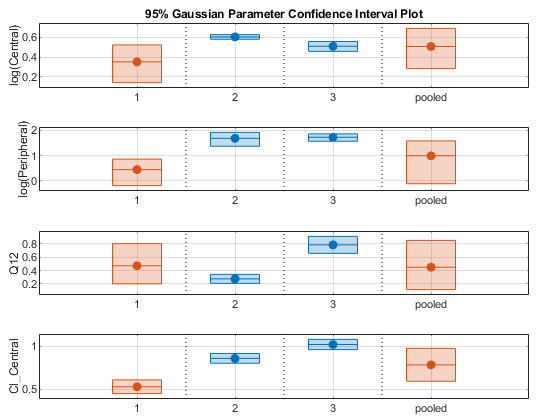
You can also plot all confidence intervals in one axes grouped by parameter estimates using the 'Grouped' layout.

plot(ciAll,'Layout','Grouped')

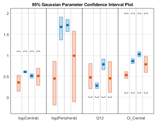
In this layout, you can point to the center marker of each confidence interval to see the group name. Each estimated parameter is separated by a vertical black line. Vertical dotted lines group confidence intervals of parameter estimates that were computed in a common fit. Parameter bounds defined in the original fit are marked by square brackets. Note the different scales on the y-axis due to parameter transformations. For instance, the y-axis of Q12 is in the linear scale, but that of Central is in the log scale due to its log transform.

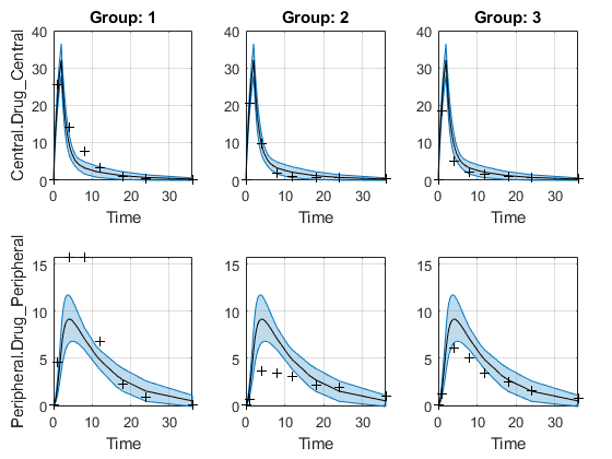
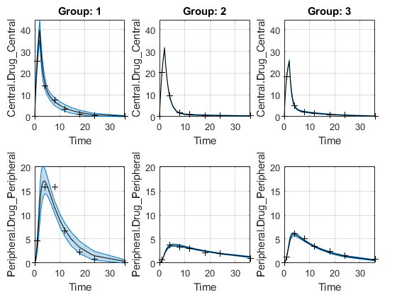
Compute Confidence Intervals for Model Predictions

Calculate 95% confidence intervals for the model predictions, that is, simulation results using the estimated parameters.

% For the pooled fit
ciPredPooled = sbiopredictionci(pooledFit);
% For the unpooled fit
ciPredUnpooled = sbiopredictionci(unpooledFit);

Plot Confidence Intervals for Model Predictions

The confidence interval for each group is plotted in a separate column, and each response is plotted in a separate row. Confidence intervals limited by the bounds are plotted in red. Confidence intervals not limited by the bounds are plotted in blue.

plot(ciPredPooled)

plot(ciPredUnpooled)