Estimate Category-Specific PK Parameters for Multiple Individuals
This example shows how to estimate category-specific (such as young versus old, male versus female), individual-specific, and population-wide parameters using PK profile data from multiple individuals.
Background
Suppose you have drug plasma concentration data from 30 individuals and want to estimate pharmacokinetic parameters, namely the volumes of central and peripheral compartment, the clearance, and intercompartmental clearance. Assume the drug concentration versus the time profile follows the biexponential decline , where is the drug concentration at time t, and and are slopes for corresponding exponential declines.
Load Data
This synthetic data contains the time course of plasma concentrations of 30 individuals after a bolus dose (100 mg) measured at different times for both central and peripheral compartments. It also contains categorical variables, namely Sex and Age.
clear
load('sd5_302RAgeSex.mat')
Convert to groupedData Format
Convert the data set to a groupedData object, which is the required data format for the fitting function sbiofit. A groupedData object also allows you set independent variable and group variable names (if they exist). Set the units of the ID, Time, CentralConc, PeripheralConc, Age, and Sex variables. The units are optional and only required for the UnitConversion feature, which automatically converts matching physical quantities to one consistent unit system.
gData = groupedData(data);
gData.Properties.VariableUnits = {'','hour','milligram/liter','milligram/liter','',''};
gData.Properties
ans = struct with fields:
Description: ''
UserData: []
DimensionNames: {'Row' 'Variables'}
VariableNames: {'ID' 'Time' 'CentralConc' 'PeripheralConc' 'Sex' 'Age'}
VariableTypes: ["double" "double" "double" "double" "categorical" "categorical"]
VariableDescriptions: {}
VariableUnits: {'' 'hour' 'milligram/liter' 'milligram/liter' '' ''}
VariableContinuity: []
RowNames: {}
CustomProperties: [1×1 matlab.tabular.CustomProperties]
GroupVariableName: 'ID'
IndependentVariableName: 'Time'
The IndependentVariableName and GroupVariableName properties have been automatically set to the Time and ID variables of the data.
Visualize Data
Display the response data for each individual.
t = sbiotrellis(gData,'ID','Time',{'CentralConc','PeripheralConc'},...
                'Marker','+','LineStyle','none');
% Resize the figure.
t.hFig.Position(:) = [100 100 1280 800];

Set Up a Two-Compartment Model
Use the built-in PK library to construct a two-compartment model with infusion dosing and first-order elimination where the elimination rate depends on the clearance and volume of the central compartment. Use the configset object to turn on unit conversion.
pkmd                                    = PKModelDesign;
pkc1                                    = addCompartment(pkmd,'Central');
pkc1.DosingType                         = 'Bolus';
pkc1.EliminationType                    = 'linear-clearance';
pkc1.HasResponseVariable                = true;
pkc2                                    = addCompartment(pkmd,'Peripheral');
model                                   = construct(pkmd);
configset                               = getconfigset(model);
configset.CompileOptions.UnitConversion = true;
For details on creating compartmental PK models using the SimBiology® built-in library, see Create Pharmacokinetic Models.
Define Dosing
Assume every individual receives a bolus dose of 100 mg at time = 0. For details on setting up different dosing strategies, see Doses in SimBiology Models.
dose             = sbiodose('dose','TargetName','Drug_Central');
dose.StartTime   = 0;
dose.Amount      = 100;
dose.AmountUnits = 'milligram';
dose.TimeUnits   = 'hour';
Map the Response Data to Corresponding Model Components
The data contains measured plasma concentration in the central and peripheral compartments. Map these variables to the appropriate model components, which are Drug_Central and Drug_Peripheral.
responseMap = {'Drug_Central = CentralConc','Drug_Peripheral = PeripheralConc'};Specify Parameters to Estimate
Specify the volumes of central and peripheral compartments Central and Peripheral, intercompartmental clearance Q12, and clearance Cl_Central as parameters to estimate. The estimatedInfo object lets you optionally specify parameter transforms, initial values, and parameter bounds. Since both Central and Peripheral are constrained to be positive, specify a log-transform for each parameter.
paramsToEstimate    = {'log(Central)', 'log(Peripheral)', 'Q12', 'Cl_Central'};
estimatedParam      = estimatedInfo(paramsToEstimate,'InitialValue',[1 1 1 1]);
Estimate Individual-Specific Parameters
Estimate one set of parameters for each individual by setting the 'Pooled' name-value pair argument to false.
unpooledFit = sbiofit(model,gData,responseMap,estimatedParam,dose,'Pooled',false);Display Results
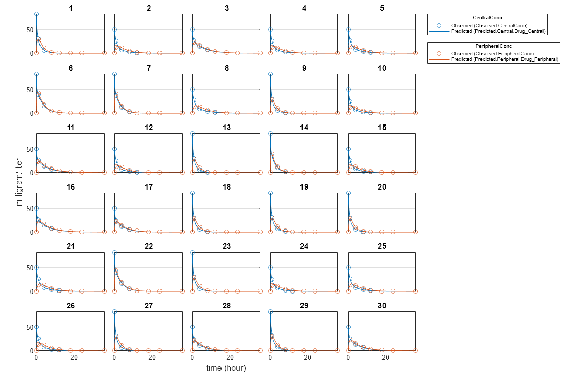
Plot the fitted results versus the original data for each individual (group).
plot(unpooledFit);

For an unpooled fit, sbiofit always returns one results object for each individual.
Examine Parameter Estimates for Category Dependencies
Explore the unpooled estimates to see if there is any category-specific parameters, that is, if some parameters are related to one or more categories. If there are any category dependencies, it might be possible to reduce the number of degrees of freedom by estimating just category-specific values for those parameters.
First extract the ID and category values for each ID
catParamValues = unique(gData(:,{'ID','Sex','Age'}));Add variables to the table containing each parameter's estimate.
allParamValues            = vertcat(unpooledFit.ParameterEstimates);
catParamValues.Central    = allParamValues.Estimate(strcmp(allParamValues.Name, 'Central'));
catParamValues.Peripheral = allParamValues.Estimate(strcmp(allParamValues.Name, 'Peripheral'));
catParamValues.Q12        = allParamValues.Estimate(strcmp(allParamValues.Name, 'Q12'));
catParamValues.Cl_Central = allParamValues.Estimate(strcmp(allParamValues.Name, 'Cl_Central'));
Plot estimates of each parameter for each category. gscatter requires Statistics and Machine Learning Toolbox™. If you do not have it, use other alternative plotting functions such as plot.
h           = figure;
ylabels     = ["Central","Peripheral","Q12","Cl\_Central"];
plotNumber  = 1;
for i = 1:4
    thisParam = estimatedParam(i).Name;

    % Plot for Sex category
    subplot(4,2,plotNumber);
    plotNumber  = plotNumber + 1;
    gscatter(double(catParamValues.Sex), catParamValues.(thisParam), catParamValues.Sex);
    ax          = gca;
    ax.XTick    = [];
    ylabel(ylabels(i));
    legend('Location','bestoutside')
    % Plot for Age category
    subplot(4,2,plotNumber);
    plotNumber  = plotNumber + 1;
    gscatter(double(catParamValues.Age), catParamValues.(thisParam), catParamValues.Age);
    ax          = gca;
    ax.XTick    = [];
    ylabel(ylabels(i));
    legend('Location','bestoutside')
end
% Resize the figure.
h.Position(:) = [100 100 1280 800];

Based on the plot, it seems that young individuals tend to have higher volumes of central and peripheral compartments (Central, Peripheral) than old individuals (that is, the volumes seem to be age-specific). In addition, males tend to have lower clearance rates (Cl_Central) than females but the opposite for the Q12 parameter (that is, the clearance and Q12 seem to be sex-specific).
Estimate Category-Specific Parameters
Use the 'CategoryVariableName' property of the estimatedInfo object to specify which category to use during fitting. Use 'Sex' as the group to fit for the clearance Cl_Central and Q12 parameters. Use 'Age' as the group to fit for the Central and Peripheral parameters.
estimatedParam(1).CategoryVariableName = 'Age';
estimatedParam(2).CategoryVariableName = 'Age';
estimatedParam(3).CategoryVariableName = 'Sex';
estimatedParam(4).CategoryVariableName = 'Sex';
categoryFit = sbiofit(model,gData,responseMap,estimatedParam,dose)
categoryFit =
  OptimResults with properties:

                   ExitFlag: 3
                     Output: [1×1 struct]
                  GroupName: []
                       Beta: [8×5 table]
         ParameterEstimates: [120×6 table]
                          J: [240×8×2 double]
                       COVB: [8×8 double]
           CovarianceMatrix: [8×8 double]
                          R: [240×2 double]
                        MSE: 0.4362
                        SSE: 205.8690
                    Weights: []
              LogLikelihood: -477.9195
                        AIC: 971.8390
                        BIC: 1.0052e+03
                        DFE: 472
             DependentFiles: {1×3 cell}
                       Data: [240×6 groupedData]
    EstimatedParameterNames: {'Central'  'Peripheral'  'Q12'  'Cl_Central'}
             ErrorModelInfo: [1×3 table]
         EstimationFunction: 'lsqnonlin'
When fitting by category (or group), sbiofit always returns one results object, not one for each category level. This is because both male and female individuals are considered to be part of the same optimization using the same error model and error parameters, similarly for the young and old individuals.
Plot Results
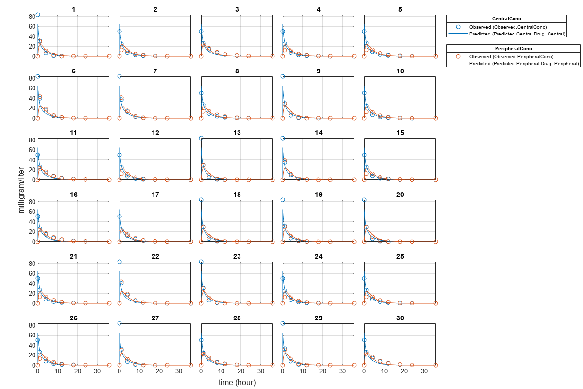
Plot the category-specific estimated results.
plot(categoryFit);

For the Cl_Central and Q12 parameters, all males had the same estimates, and similarly for the females. For the Central and Peripheral parameters, all young individuals had the same estimates, and similarly for the old individuals.
Estimate Population-Wide Parameters
To better compare the results, fit the model to all of the data pooled together, that is, estimate one set of parameters for all individuals by setting the 'Pooled' name-value pair argument to true. The warning message tells you that this option will ignore any category-specific information (if they exist).
pooledFit = sbiofit(model,gData,responseMap,estimatedParam,dose,'Pooled',true);Warning: CategoryVariableName property of the estimatedInfo object is ignored when using the 'Pooled' option.
Plot Results
Plot the fitted results versus the original data. Although a separate plot was generated for each individual, the data was fitted using the same set of parameters (that is, all individuals had the same fitted line).
plot(pooledFit);

Compare Residuals
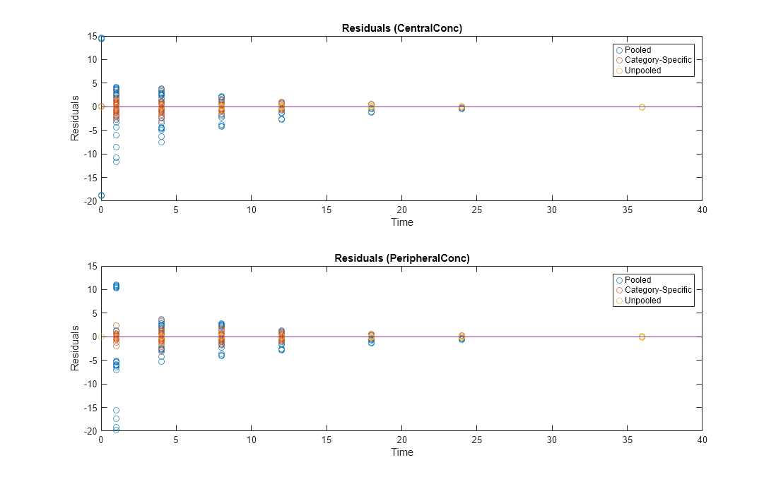
Compare residuals of CentralConc and PeripheralConc responses for each fit.
t = gData.Time;
allResid(:,:,1) = pooledFit.R;
allResid(:,:,2) = categoryFit.R;
allResid(:,:,3) = vertcat(unpooledFit.R);

h = figure;
responseList = {'CentralConc', 'PeripheralConc'};
for i = 1:2
    subplot(2,1,i);
    oneResid = squeeze(allResid(:,i,:));
    plot(t,oneResid,'o');
    refline(0,0); % A reference line representing a zero residual
    title(sprintf('Residuals (%s)', responseList{i}));
    xlabel('Time');
    ylabel('Residuals');
    legend({'Pooled','Category-Specific','Unpooled'});
end
% Resize the figure.
h.Position(:) = [100 100 1280 800];
As shown in the plot, the unpooled fit produced the best fit to the data as it fit the data to each individual. This was expected since it used the most number of degrees of freedom. The category-fit reduced the number of degrees of freedom by fitting the data to two categories (sex and age). As a result, the residuals were larger than the unpooled fit, but still smaller than the population-fit, which estimated just one set of parameters for all individuals. The category-fit might be a good compromise between the unpooled and pooled fitting provided that any hierarchical model exists within your data.