Find Important Tumor Growth Parameters with Local Sensitivity Analysis Using SimBiology Model Analyzer

Open Live Script

This example shows how to identify important model parameters for a tumor growth model [1]. In this example, you compute local time-dependent sensitivities of tumor growth with respect to model parameters for an anticancer drug.

Tumor Growth Model

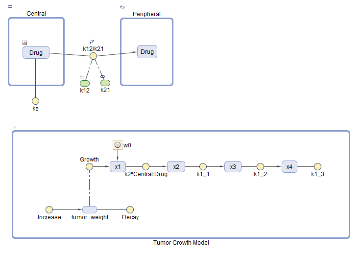
The model used in this example is a SimBiology® implementation of the pharmacokinetic/pharmacodynamic (PK/PD) model by Simeoni et al. It quantifies the effect of anticancer drugs on tumor growth kinetics from in vivo animal studies. The drug pharmacokinetics are described by a two-compartment model with IV bolus dosing and linear elimination (ke) from the Central compartment. Tumor growth is a biphasic process with an initial exponential growth followed by linear growth. The growth rate of the proliferating tumor cells is described by

$\frac{L_{0} \times x_{1}}{{[1 + {(\frac{L_{0}}{L_{1}} \times w)}^{ψ}]}^{\frac{1}{ψ}}}$

L0, L1, and Ψ are tumor growth parameters, x1 is the weight of the proliferating tumor cells, and w is the total tumor weight. In the absence of any drugs, the tumor consists of proliferating cells only, that is, w = x1. In the presence of an anticancer agent, a fraction of the proliferating cells is transformed into nonproliferating cells. The rate of this transformation is assumed to be a function of the drug concentration in the plasma and an efficacy factor k2. The nonproliferating cells x2 go through a series of transit stages (x3 and x4) and are eventually cleared from the system. The flow-through of the transit compartments is modeled as a first-order process with the rate constant k1.

The SimBiology model makes these adjustments to the pharmacodynamics of tumor growth:

Instead of defining the tumor weight as the sum of x1, x2, x3, and x4, the model defines the tumor weight by the reaction named Increase, null → tumor_weight, with the reaction rate $(\frac{2 \times L_{1} \times L_{0} \times x_{1}^{2}}{L_{1} + 2 \times L_{0} \times x_{1}}) \times tumor_weight$ . tumor_weight is the total tumor weight, x1 is the weight of the proliferating tumor cells, and L0, and L1 are tumor growth parameters [2].
Similarly, the model defines the decrease in tumor weight by the reaction named Decay, tumor_weight → null, with the reaction rate k1*x4. The constant k1 is the forward rate parameter, and x4 is the last species in the series of transit reductions in tumor weight.
ke is a function of the clearance and the volume of the central compartment: ke = Cl_Central/Central.

Local Sensitivity Analysis

Sensitivity Analysis in SimBiology lets you determine which rate constants and concentrations in a model have significant influence on the overall behavior of the model. This example shows how to investigate which model parameters are sensitive to the tumor growth using the built-in local sensitivity analysis program. Specifically, this example shows you how to calculate the local sensitivity of tumor_weight species with respect to the model parameters as follows:

$\frac{\partial (t u m o r_w e i g h t)}{\partial (L_{0})}, \frac{\partial (t u m o r_w e i g h t)}{\partial (L_{1})}, \frac{\partial (t u m o r_w e i g h t)}{\partial (k_{1})}, . . .$

Calculate Local Sensitivities

Suppose that you have already calbirated tumor growth model parameters to experimental PK/PD data and saved parameter estimates and initial conditions as a variant called parameterEstimates in your model (as shown in this example Calculate NCA Parameters and Fit Model to PK/PD Data Using SimBiology Model Analyzer). As a follow-up analysis, you want to find out which model parameters are sensitive to tumor growth. The following steps show how to do so using the built-in local sensitivity analysis program. For a global sensitivity analysis example, see Find Important Parameters for Receptor Occupancy with Global Sensitivity Analysis Using SimBiology Model Analyzer.

Load Tumor Growth Model and Data

Enter the following command to open the tumor growth model in the SimBIology Model Analyzer app.

openExample('simbio/FindTumorGrowthParametersLSASimBiologyAnalyzerExample')

Configure Calculate Sensitivities Program

First open the example. The SimBiology Model Analyzer app opens with the Tumor Growth Model model loaded.

On the Home tab, select Program > Calculate Sensitivities. A new program opens.

In the Variants section, select parameterEstimates. This variant contains previously estimated parameter values and initial conditions for the drug.

In the Doses section, select interval_dose. This repeat dose applies 30 mg of the drug every 4 days starting at day 7 for a total of five times.

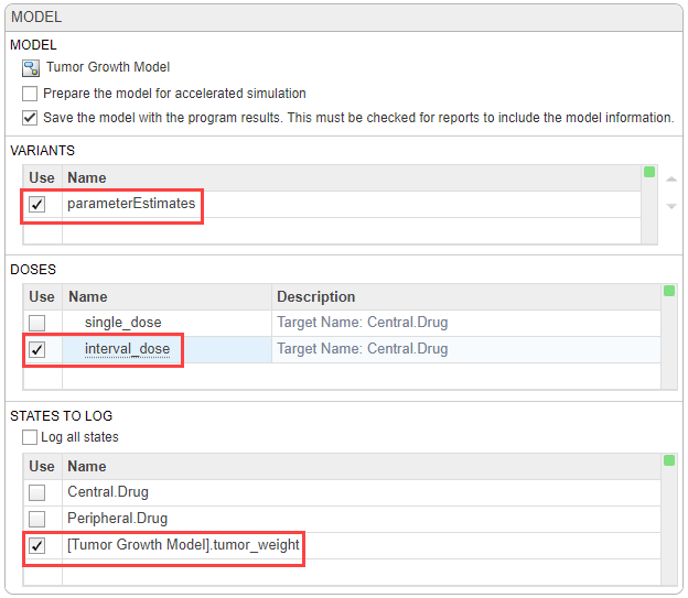
In the States To Log section, select [Tumor Growth Model].tumor_weight only.

Tip: The context menus of the Variants, Doses and States To Log tables contain options to add the corresponding model components and show the details of these components in the Model Builder app. Access the context menu by right-clicking the table.

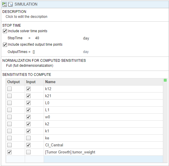
In the Simulation step, by default, the normalization method is set to Full (full dedimensionalization), meaning that the app fully normalize the sensitivities so that they can be compared to each other. For details, see Normalization. Use the default stop time (40).

Tip: You can run every program execution step separately. An execution step includes the run button next to the name the step. Running an individual step is especially helpful if the program contains multiple steps and you want to see the intermediate results from a particular step. By doing so, you can make adjustments as needed before running the next step or the whole program. To run the whole program, click the Run button on the Home tab.

In the Sensitivities to Compute section, right-click anywhere in the table and select Add All Constant Parameters. Clear ke because it is defined as a function of the Central volume and Cl_Central, which is already an input. Click the last empty row and type tumor. Then select [Tumor Growth Model].tumor_weight from the list. The tumor_weight species is then added as the output.

Check Initial Conditions

You can view the initial conditions of model quantities, namely compartments, species, and parameters, before simulating a model. The initial conditions are the quantity values at simulation time = 0 after applying the assignment rules, variants, and doses (if any at time = 0). For details, see Model Simulation. You can use this information to debug a model and check if the quantity values are initialized as you expect before simulating the model.

In the Browser pane, click Model.

Right-click anywhere within the Species and Compartments table or Parameters table. Select Show Model Initial Conditions.

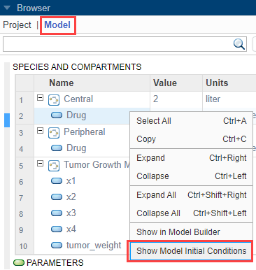
The app shows the Initial Condition column in both quantity tables. These values are what the program uses at time = 0 when you simulate.

Next, run the program by clicking Run on the Home tab.

Visualize Sensitivity Results

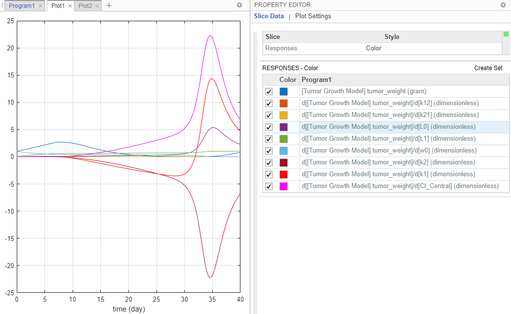
After the sensitivity analysis, the program automatically generates two plot tabs Plot1 and Plot2. Click Plot1 to view a plot of the time course of the tumor weight and other sensitivity values d[tumor_weight]/d[parameter]. The time plots for d[tumor_weight]/d[k21] and d[tumor_weight]/d[k12] stay relatively flat compared to other sensitivities, indicating that the tumor growth is not sensitive to k21 and k12 parameters. The Property Editor lets you select which plots to display.

Tip: Plots are backed by data that are currently present in the app workspace. Plots are not snapshots. When the data (either experimental data or simulation results) is removed or changed, the plots are also updated according to the changes in the underlying data.

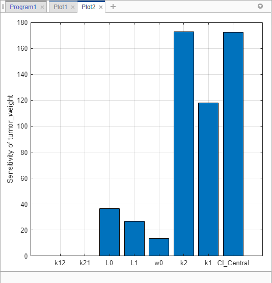
You can also examine the same sensitivity data by checking the magnitude of the computed sensitivities integrated over time. The second generated plot (Plot2) shows a bar plot containing such information. The plot shows that the tumor weight is sensitive to L0, L1, w0, k2, k1, and Cl_Central, but not to k12 and k21.

Save the sensitivity analysis results in a separate folder.

Click Project in the Browser pane. Expand the Program1 folder.
Right-click the LastRun folder. Select Save Data.
In the Save Data dialog, enter sa_data as the data name.

Investigate Variability of k12 and k21

First, vary values for the k12 parameter. Click the Program1 tab. Click the (+) plus at the top of the program and select Generate Samples.

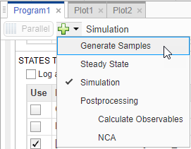
The Generate Samples step appears. Disable the default plot generation by clicking the plot button at the top of the step.

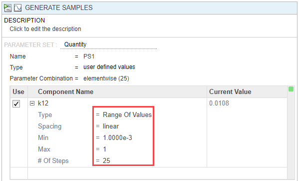
In the Parameter Set section of the step, double-click the empty cell in the Component Name, and enter k12. Set the following options:

Type — Range Of Values
Spacing — linear
Min — 1e-3
Max — 1
# Of Steps — 25

In the Simulation step, under Sensitivities to Compute, clear all the inputs except k12. Keep tumor_weight as the output. Also, disable the default plot generation by clicking the plot button at the top of the step.

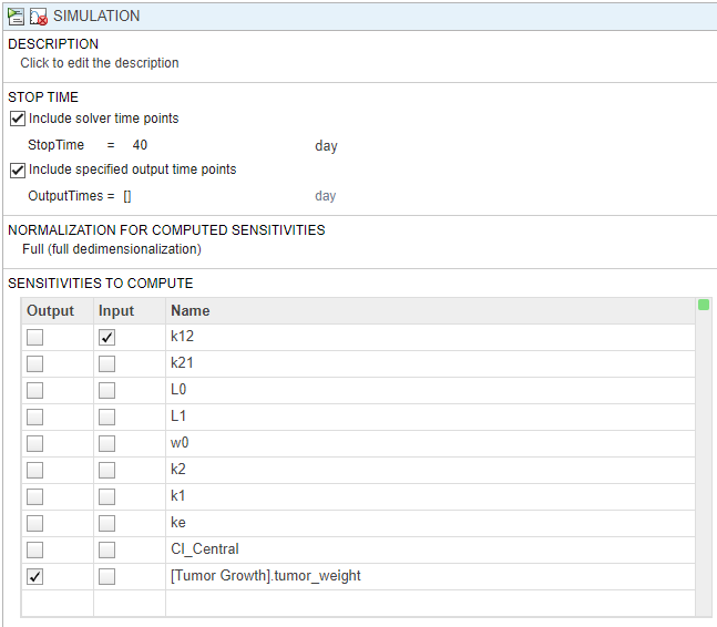
On the Home tab, click the Run button to run the whole program.

Once the simulation finishes, the sensitivity results are stored in the LastRun folder. Expand the LastRun folder. Click results. Then select time from the Plot section on the Home tab. The Responses in the plot correspond to the tumor weight and the sensitivity of the tumor weight with respect to k12. Each response is plotted using a different line style. The Scenarios correspond to each parameter scan (simulation scenario). Each scenario is plotted using a different color.

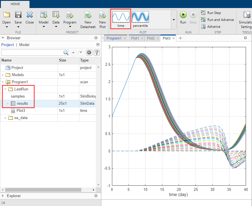
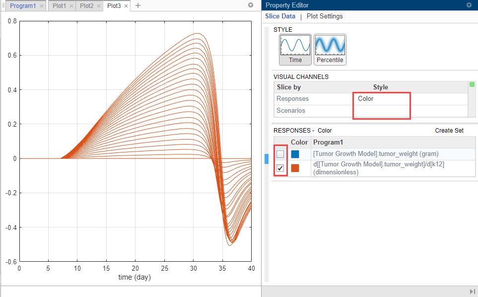
Customize the plot so that the plot uses a different color for each response instead. In the Slice Data table, clear the Style of Scenarios by selecting empty. Set Responses to Color.

In the Responses table, clear tumor_weight and keep only the sensitivity results. The plot suggests that the tumor weight is sensitive to some k12 parameter values when model variants different than the estimated parameter values are explored.

Plot the k12 sensitivities together with the previous sensitivity results to see how sensitive the tumor growth is to k12 relative to other model parameters. In the Browser pane, expand the folder sa_data that you saved previously. Then expand results.

Multiselect (Shift + Click) the sensitivity data entries for L0, L1, w0, k2, k1, and Cl_Central. Then drag them on to the k12 sensitivity plot Plot3. The plot suggests that the tumor growth is still more sensitive to most of the other parameters than k12.

Save the results in a separate folder. Right-click LastRun and select Save Data. Enter k12_data as the data name.

Vary k21

You can perform a similar analysis by varying k21 and comparing its results with other parameter sensitivities.

Return to Program1. In the Generate Samples step, click Add parameter set to scan. A new Parameter Set section appears.

Double-click the empty cell in the Component Name, and enter k21. Set the same options as k12:

Type — Range of Values
Spacing — linear
Min — 1e-3
Max — 1
# Of Steps — 25

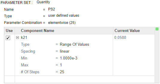
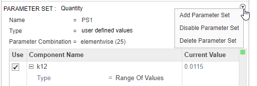
Disable the first parameter set (PS1). Point to the top corner of Parameter Set section of PS1 and click the action button. Then select Disable Parameter Set.

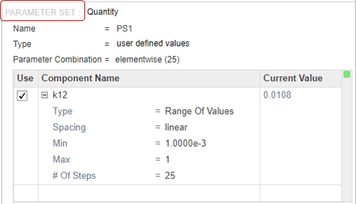
The Parameter Set is then grayed out to indicate you have successfully disabled it.

In the Simulation step, select k21 as the only input and tumor_weight as the output.

Hit Run from the Home tab to run the program again.

Once the simulation finishes, the results are automatically plotted in a new plot tab.

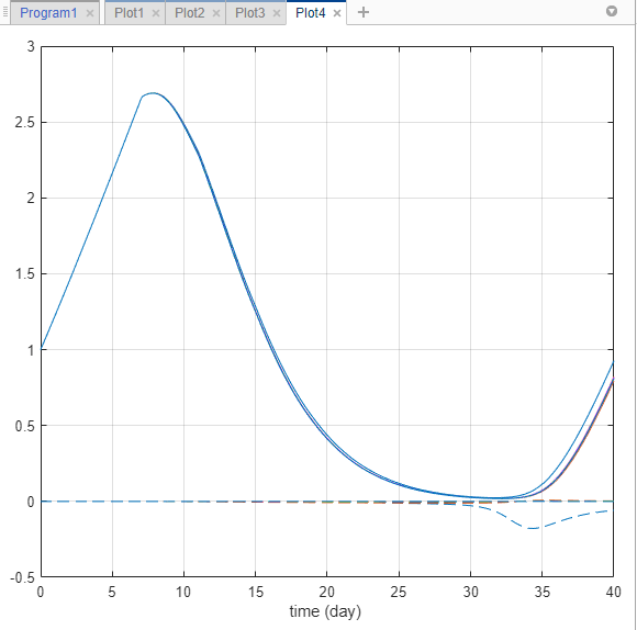
In the Slice Data table, clear the Style of Scenarios by selecting empty. Set Responses to Color.

In the Responses table, clear tumor_weight and keep only the sensitivity results. The plot suggests that the tumor weight is sensitive to some k21 parameter values when model variants different than the estimated parameter values are explored.

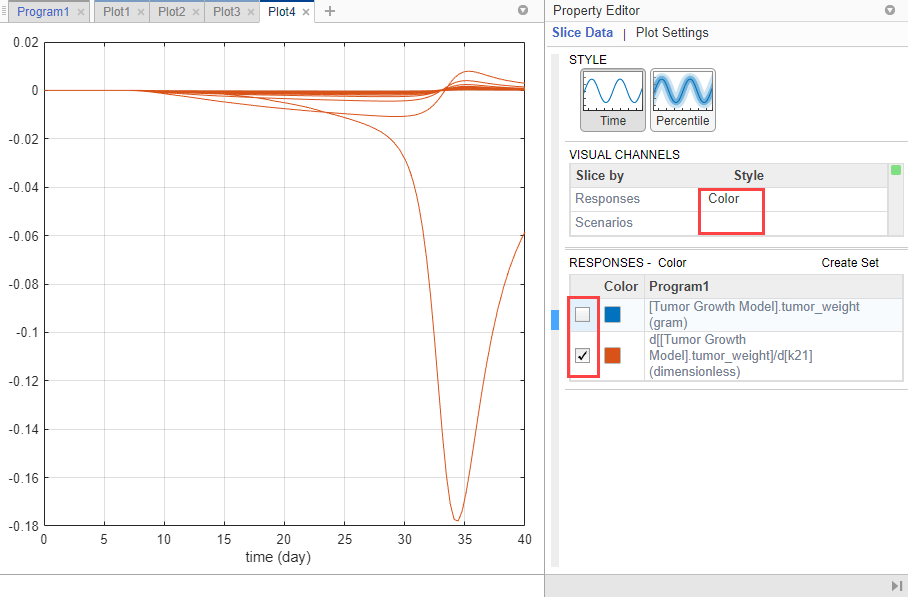
Plot k21 sensitivities together with the previous sensitivity results to compare. Click Plot3. In the Browser pane, expand the LastRun folder. Then expand results.

Drag the k21 sensitivity data d[[Tumor Growth Model].tumor_weight]/d[k21] on to Plot3. The plot suggests that the tumor growth is relatively more sensitive to most other parameters than k21 and k12.

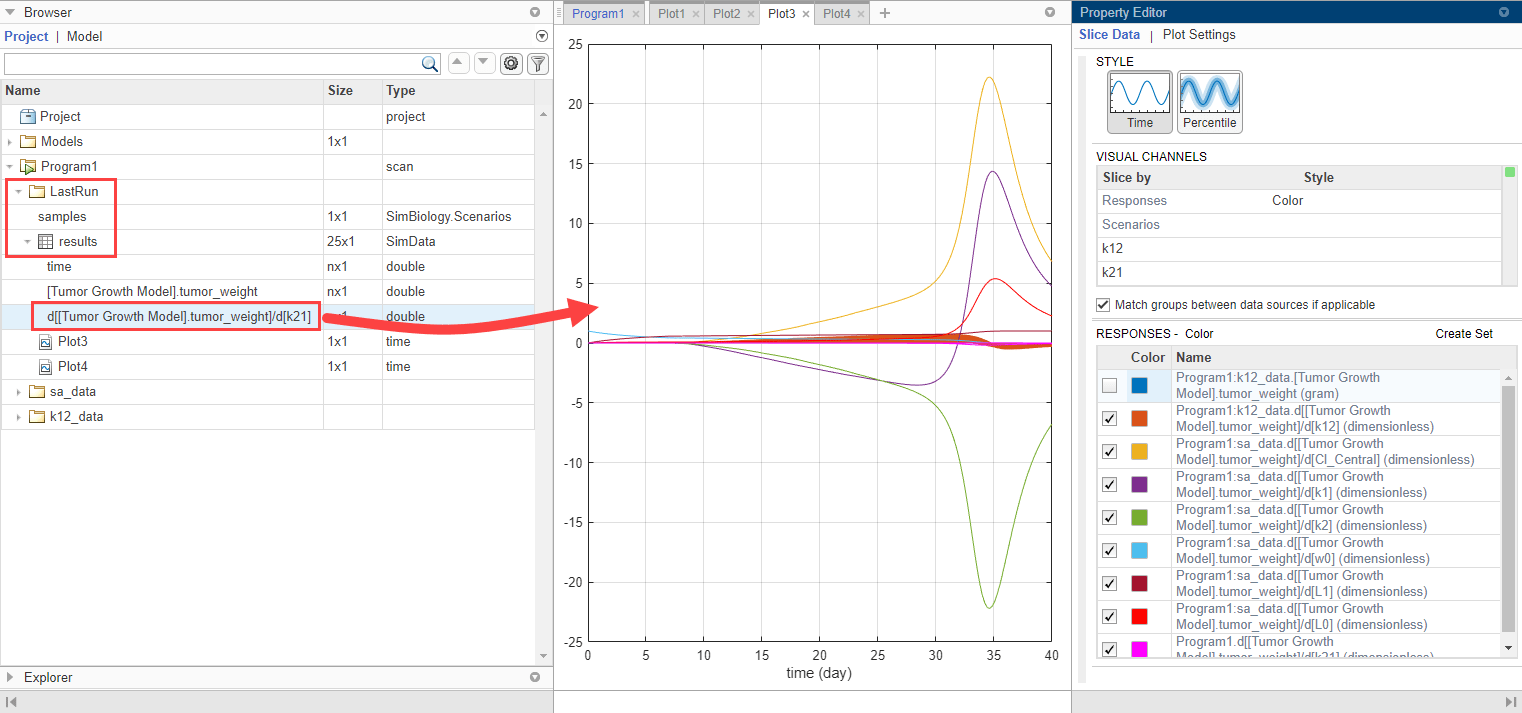
This example shows how to perform sensitivity analysis to find important model parameters to which tumor growth is sensitive. The initial analysis concludes that the tumor weight is not sensitive to some of the parameters. The example then explores the parameter space of these less sensitive parameters and compares the sensitivity results with those of other model parameters. You can use such sensitivity information for other analyses, such as to perform Explore Biological Variability with Virtual Patients Using SimBiology Model Analyzer by varying sensitive parameters to explore the model dynamics and biological variability.

References

[1] Simeoni, Monica, Paolo Magni, Cristiano Cammia, Giuseppe De Nicolao, Valter Croci, Enrico Pesenti, Massimiliano Germani, Italo Poggesi, and Maurizio Rocchetti. “Predictive Pharmacokinetic-Pharmacodynamic Modeling of Tumor Growth Kinetics in Xenograft Models after Administration of Anticancer Agents.” Cancer Research 64, no. 3 (February 1, 2004): 1094–1101.

[2] Koch, Gilbert, Antje Walz, Gezim Lahu, and Johannes Schropp. “Modeling of Tumor Growth and Anticancer Effects of Combination Therapy.” Journal of Pharmacokinetics and Pharmacodynamics 36, no. 2 (April 2009): 179–97.