Definitions and Evaluations of Rules in SimBiology Models

Overview

Rules are mathematical expressions that allow you to define or modify model quantities, namely compartment capacity, species amount, or parameter value.

Rules can take the form of initial assignments, assignments during the course of a simulation (repeated assignments), algebraic relationships, or differential equations (rate rules). Details of each type of rule are described next.

Initial Assignment

An initial assignment rule lets you specify the initial value of a model quantity as a numeric value or as a function of other model quantities. It is evaluated once at the beginning of a simulation.

An initial assignment rule is expressed as Variable = Expression, and the rule is specified as the Expression. For example, you could write an initial assignment rule to set the initial amount of species2 to be proportional to species1 as species2 = k * species1 where k is a constant parameter.

Repeated Assignment

A repeated assignment rule lets you specify the value of a quantity as a numeric value or as a function of other quantities repeatedly during the simulation. It is evaluated at every time step, which is determined by the solver during the simulation process.

A repeated assignment rule is expressed as Variable = Expression, and the rule is specified as the Expression. For example, to repeatedly evaluate the total species amount by summing up the species in different compartments, you could enter: xTotal = c1.X + c2.X, where xTotal is a nonconstant parameter, c1 and c2 are the name of compartments where species x resides.

Algebraic Rules

An algebraic rule lets you specify mathematical constraints on one or more model quantities that must hold during a simulation. It is evaluated continuously during a simulation.

An algebraic rule takes the form 0 = Expression, and the rule is specified as the Expression. For example, if you have a mass conservation equation such as species_total = species1 + species2, write the corresponding algebraic rule as species1 + species2 - species_total.

However, repeated assignment rules are mathematically equivalent to algebraic rules, but result in exact solutions instead of approximated solutions. Therefore, it is recommended that you use repeated assignment rules instead of algebraic rules whenever possible. Use algebraic rules only when:

You cannot analytically solve the equations to get a closed-form solution. For example, there is no closed-form solution for x^4 + ax^3 + bx^2 + cx + k = 0 whereas the closed-form solution for kx – c = 0 is x = c/k.
You have multiple equations with multiple unknowns, and they could be inconvenient to solve.

If you use an algebraic rule, rate rule, or repeated assignment to vary the value of a parameter or compartment during the simulation, make sure the ConstantValue property of the parameter or ConstantCapacity of the compartment is set to false.

Repeated Assignment vs. Algebraic Rules

Repeated assignment rules are mathematically equivalent to algebraic rules, but result in exact solutions. However, algebraic rules are solved numerically, and the accuracy depends on the error tolerances specified in the simulation settings. In addition, there are several advantages to repeated assignment rules such as better computational performance, more accurate results since no rules have to be solved numerically (hence no approximations), and sensitivity analysis support.

Tip

If you can analytically solve for a variable, use a repeated assignment rule instead of an algebraic rule.
In repeated assignment rules, the constrained variable is explicitly defined as the left-hand side, whereas in algebraic rules it is inferred from the degrees of freedom in the system of equations. See also Considerations When Imposing Constraints.

Rate Rules

A rate rule represents a differential equation and lets you specify the time derivative of a model quantity. It is evaluated continuously during a simulation.

A rate rule is represented as $\frac{d V a r i a b l e}{d t} = E x p r e s s i o n$ , which is expressed in SimBiology as Variable = Expression. For example, if you have a differential equation for species x, $\frac{d x}{d t} = k (y + z)$ , write the rate rule as: x = k * (y + z).

For more examples, see Rate Rule Examples.

Evaluation Order of Rules

At the start of the simulation (that is, at simulation time = 0), SimBiology^® evaluates the initial assignment and repeated assignment rules as a set of simultaneous constraints. SimBiology treats the rules as a unified system of constraints and automatically reorders and evaluates them. The order in which the rules appear in the model has no effect on the simulation results.

If a quantity is being modified by an assignment rule, the rule replaces initial value properties, such as InitialAmount, Capacity, or Value. Similarly, a variant altering such quantities has no effect because the value is superseded by the assignment rules.

SimBiology throws an error if the model has circular dependencies in the initial assignment and repeated assignment rules. In other words, initial assignments and repeated assignments cannot have a variable that is explicitly or implicitly referenced on both the left- and right-hand sides of the equation.

For instance, you cannot create circular sets of assignments such as a = b + 1 and b = a + 1, where a and b are explicitly referenced on both sides of the equation. An example of an implicit reference is when an assignment rule references a species in concentration. In this case, the compartment that contains the species is implicitly referenced.

Warning

You might observe different simulation results with respect to initial assignments for previous releases of SimBiology (R2017a or earlier). To recover the same simulation results at time = 0, as in R2017a or earlier, use the updateInitialAssignments function in the command line. If you are using the SimBiology app, right-click the model from the Project Workspace and select Remove Order Dependencies.

Conservation of Amounts During Simulation

During a simulation (that is, at simulation time > 0), SimBiology conserves species amounts rather than concentrations if there are any changes to the volume of a compartment where the species reside. In other words, if you have a repeated assignment rule or an event that changes the volume, then you see the effect of conservation of species amounts at time > 0.

However, at the beginning of a simulation (that is, at simulation time = 0), the concept of amount conservation does not apply because there are no changes before time = 0. Only one set of initial conditions exists and SimBiology uses the conditions at the start of the simulation. Specifically, at time = 0, SimBiology:

Initializes variables for species, compartments, and parameters using the corresponding InitialAmount, Capacity, and Value properties.
Updates the values by replacing them with the corresponding alternate values from variants, if any.
Updates the values by evaluating initial assignment and repeated assignment rules as a set of simultaneous constraints. Therefore, the assignment rules replace initial values if model quantities are being modified by such rules or variants.

Warning

In previous releases (R2017a or earlier), if a repeated assignment changed a compartment volume, SimBiology used the compartment capacity to determine the initial amount and conserved it when the compartment volume changed at time = 0. In R2017b or later, SimBiology uses the InitialAmount property of the species as the initial condition at time = 0. Consider the following model.

m = sbiomodel('m1')
v = addcompartment(m,'v',10,'ConstantCapacity',0,'CapacityUnit','liter')
p = addparameter(m,'p','ValueUnit','liter')
r = addrule(m,'v = 100 * p','repeatedAssignment')
s = addspecies(v,'s',50,'InitialAmountUnit','milligram/liter')

In R2017a or earlier, SimBiology first calculated the initial amount of s as

50 milligram/liter * 10 liter = 500
                        milligram

, and then applied the repeated assignment rule v = 100 liter. So, the concentration of s was then calculated and reported as

500
                        milligram/100 liter = 5 milligram/liter

at time = 0.

In R2017b or later, SimBiology uses the InitialAmount property of species s, and reports the initial amount of s as 50 milligram/liter instead.

Writing Rule Expressions

Use MATLAB^® syntax to write a mathematical expression for a rule. Note that no semicolon or comma is needed at the end of a rule expression. If your algebraic, repeated assignment, or rate rule expression is not continuous or differentiable, see Using Events to Address Discontinuities in Rule and Reaction Rate Expressions before simulating your model.

Considerations When Imposing Constraints

Suppose that you have a species y whose amount is determined by the equation y = m * x - c. In SimBiology, the algebraic rule to describe this constraint is written as m * x - c - y. If you want to use this rule to determine the value of y, then m, x, and c must be variables or constants whose values are known or determined by other equations. Therefore, you must ensure that the system of equations is not overconstrained or underconstrained. For instance, if you have more equations than unknowns, then the system is overconstrained. Conversely, if you have more unknowns than the equations, then the system is underconstrained.

Tip

The behavior of an underconstrained system could be fixed by adding additional rules or by setting the ConstantValue or ConstantCapacity or ConstantAmount property of some of the components in the model.

Rate Rule Examples

The following examples show how to create rate rules for different applications.

Create a Rate Rule for a Constant Rate of Change

Open Live Script

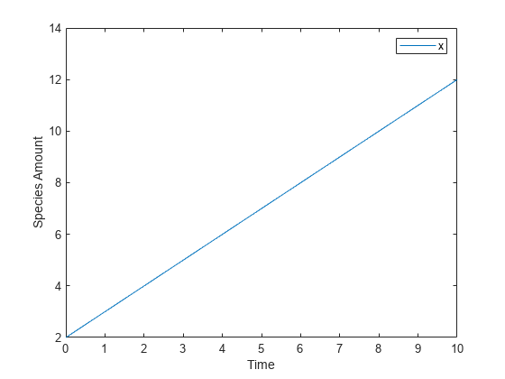
This example shows how to increase the amount or concentration of a species by a constant value using the zero-order rate rule. For example, suppose species x increases by a constant rate k. The rate of change is:

$d x / d t = k$

Set the initial amount of species x to 2, and the value of parameter k to 1. Use the following commands to set up a SimBiology model accordingly and simulate it.

m = sbiomodel('m');
c = addcompartment(m,'comp');
s = addspecies(m,'x','InitialAmount',2);
p = addparameter(m,'k','Value',1);
r = addrule(m,'x = k','RuleType','rate');
[t,sd,species] = sbiosimulate(m);
plot(t,sd);
legend(species)
xlabel('Time');
ylabel('Species Amount');

Figure contains an axes object. The axes object with xlabel Time, ylabel Species Amount contains an object of type line. This object represents x.

Alternatively, you could model a constant increase in a species using the Mass Action reaction null -> x with the forward rate constant k.

clear
m = sbiomodel('m');
c = addcompartment(m,'comp');
s = addspecies(m,'x','InitialAmount',2);
r = addreaction(m,'null -> x');
kl = addkineticlaw(r,'MassAction');
p = addparameter(kl,'k','Value',1);
kl.ParameterVariableNames = 'k';
[t,sd,species] = sbiosimulate(m);
plot(t,sd);
legend(species)
xlabel('Time');
ylabel('Species Amount');

Figure contains an axes object. The axes object with xlabel Time, ylabel Species Amount contains an object of type line. This object represents x.

Create a Rate Rule for an Exponential Rate of Change

Open Live Script

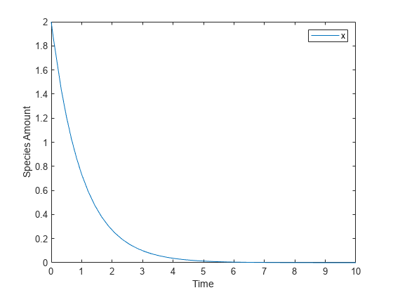
This example shows how to change the amount of a species similar to a first-order reaction using the first-order rate rule. For example, suppose the species x decays exponentially. The rate of change of species x is:

$d x / d t = - k * x$

The analytical solution is:

$C_{t} = C_{0} * e^{- k t}$

where $C_{t}$ is the amount of species at time t, and $C_{0}$ is the initial amount. Use the following commands to set up a SimBiology model accordingly and simulate it.

m = sbiomodel('m');
c = addcompartment(m,'comp');
s = addspecies(m,'x','InitialAmount',2);
p = addparameter(m,'k','Value',1);
r = addrule(m,'x = -k * x','RuleType','rate');
[t,sd,species] = sbiosimulate(m);
plot(t,sd);
legend(species);
xlabel('Time');
ylabel('Species Amount');

Figure contains an axes object. The axes object with xlabel Time, ylabel Species Amount contains an object of type line. This object represents x.

If the amount of a species x is determined by a rate rule and x is also in a reaction, x must have its BoundaryCodition property set to true. For example, with a reaction a -> x and a rate rule $\frac{d x}{d t} = k * x$ , set the BoundaryCodition property of species x to true so that a differential rate term is not created from the reaction. The amount of x is determined solely by a differential rate term from the rate rule. If the BoundaryCodition property is set to false, you will get the following error message such as Invalid rule variable 'x' in rate rule or reaction.

Create a Rate Rule to Define a Differential Rate Equation

Many mathematical models in the literature are described with differential rate equations for the species. You could manually convert the equations to reactions, or you could enter the equations as rate rules. For example, you could enter the following differential rate equation for a species C:

$\frac{dC}{dt} = vi - vdX \frac{C}{Kc + C} - kdC$

as a rate rule in SimBiology: C = vi - (vd*X*C)/(Kc + C) - kd*C

Create a Rate Rule for the Rate of Change That Is Determined by Another Species

Open Live Script

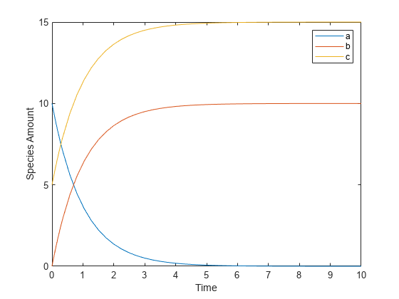
This example shows how to create a rate rule where a species from one reaction can determine the rate of another reaction if it is in the second reaction rate equation. Similarly, a species from a reaction can determine the rate of another species if it is in the rate rule that defines that other species. Suppose you have a SimBiology model with three species (a, b, and c), one reaction (a -> b), and two parameters (k1 and k2). The rate equation is defined as $b = - k_{1} * a$ , and rate rule is $d c / d t = k_{2} * a$ . The solution for the species in the reaction are:

$a = a_{o} e^{- k_{1} t}$ , $b = a_{o} (1 - e^{- k_{1} t})$ .

Since the rate rule $d c / d t = k_{2} * a$ is dependent on the reaction, $d c / d t = k_{2} (a_{o} e^{- k_{1} t})$ . The solution is:

$c = c_{o} + k_{2} a_{o} / k_{1} (1 - e^{- k_{1} t})$

Enter the following commands to set up a SimBiology model accordingly and simulate it.

m = sbiomodel('m');
c = addcompartment(m,'comp');
s1 = addspecies(m,'a','InitialAmount',10,'InitialAmountUnits','mole');
s2 = addspecies(m,'b','InitialAmount',0,'InitialAmountUnits','mole');
s3 = addspecies(m,'c','InitialAmount',5,'InitialAmountUnits','mole');
rxn = addreaction(m,'a -> b');
kl = addkineticlaw(rxn,'MassAction');
p1 = addparameter(kl,'k1','Value',1,'ValueUnits','1/second');
rule = addrule(m,'c = k2 * a','RuleType','rate');
kl.ParameterVariableNames = 'k1';
p2 = addparameter(m,'k2','Value',1,'ValueUnits','1/second');
[t,sd,species] = sbiosimulate(m);
plot(t,sd);
legend(species);
xlabel('Time');
ylabel('Species Amount');

Figure contains an axes object. The axes object with xlabel Time, ylabel Species Amount contains 3 objects of type line. These objects represent a, b, c.