Model Traffic Intersections as a Queuing Network
This example shows how to create a SimEvents® model to represent a vehicle traffic network and to investigate mean waiting time of vehicles when the network is in steady-state.
Suppose a vehicle traffic network consists of two vehicle entry and two vehicle exit points, represented by brown and green nodes in the next figure. Each blue node in the network represents a route intersection with a traffic light, and the arrows represent the route connections at each intersection. The values next to the arrows represent the percentage of vehicles taking the route in that intersection.
![]()
The rate of vehicle entries into the network are represented by the Poisson processes with rates 0.5 for Entry 1 and 0.15 for Entry 2. Service rates represent the time vehicles spend at each intersection, which are drawn from exponential distribution with mean 1. The arrow values are the probabilities of choosing a route for vehicles in the intersection.
Model Traffic Network
To represent a vehicle traffic network, this model uses Entity Generator, Entity Server, Entity Queue, Entity Input Switch, Entity Output Switch, and Entity Terminator blocks.
model = 'QueueServerTransportationNetwork';
open_system(model);

Model Vehicle Arrivals
The two Entity Generator blocks represent the network entry points. Their entity intergeneration time is set to create a Poisson arrival process.
This is the code in the Intergeneration time action field of the Entry 1 block.
% Random number generation
coder.extrinsic('rand');
ValEntry1 = 1;
ValEntry1 = rand();
% Pattern: Exponential distribution
mu = 0.5;
dt = -1/mu * log(1 - ValEntry1);
In the code, mu is the Poisson arrival rate. The coder.extrinsic('rand') is used because there is no unique seed assigned for the randomization. For more information about random number generation in event actions, see Event Action Languages and Random Number Generation. To learn more about extrinsic functions, see Working with mxArrays.
Model Vehicle Route Selection
Entities have a Route attribute that takes value 1 or 2. The value of the attribute determines the output port from which the entities depart an Entity Output Switch block.
This code in the Entry action of the Entity Server 1 represents the random route selections of vehicles at the intersection represented by Node 1.
Coin1 = 1;
coder.extrinsic('rand');
Coin1 = rand;
if Coin1 <= 0.2
    entity.Route = 1;
else
    entity.Route = 2;
end
This is an example of random Route attribute assignments when entities enter the Entity Server 1 block. The value of Route is assigned based on the value of the random variable rand that takes values between 0 and 1. Route becomes 1 if rand is less than or equal to 0.2, or 2 if rand is greater than 0.2.
Model Route Intersections
Each blue node represents a route intersection and includes an infinite capacity queue, and a server with service time drawn from an exponential distribution with mean 1.
Entity Server 1 contains this code.
% Pattern: Exponential distribution
coder.extrinsic('rand');
Val1 = 1;
Val1 = rand();
mu = 1;
dt = -mu * log(1 - Val1);
Calculate Mean Waiting Time for Vehicles in the Network
The network is constructed as an open Jackson network that satisfies these conditions.
All arriving vehicles can exit the network.
Vehicle arrivals are represented by Poisson process.
Vehicles depart an intersection as first-in first-out. The wait time in an intersection is exponentially distributed with mean
1.A vehicle departing the intersection either takes an available route or leaves the network.
The utilization of each traffic intersection queue is less than
1.
In the steady state, every queue in an open Jackson network behaves independently as an M/M/1 queue. The behavior of the network is the product of individual queues in equilibrium distributions. For more information about M/M/1 queues, see M/M/1 Queuing System.
The vehicle arrival rate for each node  is calculated using this formula.
In the formula:
 is the rate of external arrivals for node .
 is the total number of incoming arrows to node .
 is the probability of choosing the node from node
  .
.
 is the total vehicle arrival rate to node .
For all of the nodes in the network, the equation takes this matrix form.

Here,  is the routing matrix, and each element represents the probability of transition from node to node .
For the network investigated here, this is the routing matrix.
![$\theta = \left[\begin{array}{cccc} 0 & 0.2 & 0.8 & 0\\ 0 & 0 & 0.7 & 0.3\\ 0 & 0 & 0 & 0.4\\ 0 & 0 & 0 & 0 \end{array}\right]$](../../examples/simevents/win64/RandomNumberQueuingNetworkExample_eq17920314837264717250.png)
 is the vector of external arrivals to each node.
![$R = \left[\begin{array}{cccc} 0.5 & 0 & 0 & 0.15 \end{array}\right]$](../../examples/simevents/win64/RandomNumberQueuingNetworkExample_eq14098627766891924055.png)
Using these values, the mean arrival rate is calculated for each node.
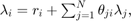
![$\lambda = \left[ \begin{array}{cccc} 0.5 & 0.1 & 0.47 & 0.368 \end{array}\right]$](../../examples/simevents/win64/RandomNumberQueuingNetworkExample_eq14265842328780400770.png)
Each node behaves as an independent M/M/1 queue, and the mean waiting time for each node is calculated by this formula. See M/M/1 Queuing System.

Mean waiting time for each node is calculated by incorporating each element of  .
.
![$\rho = \left[\begin{array}{cccc} 1 & 0.11 & 0.88 & 0.58 \end{array}\right]$](../../examples/simevents/win64/RandomNumberQueuingNetworkExample_eq18184070238554797417.png)
View Simulation Results
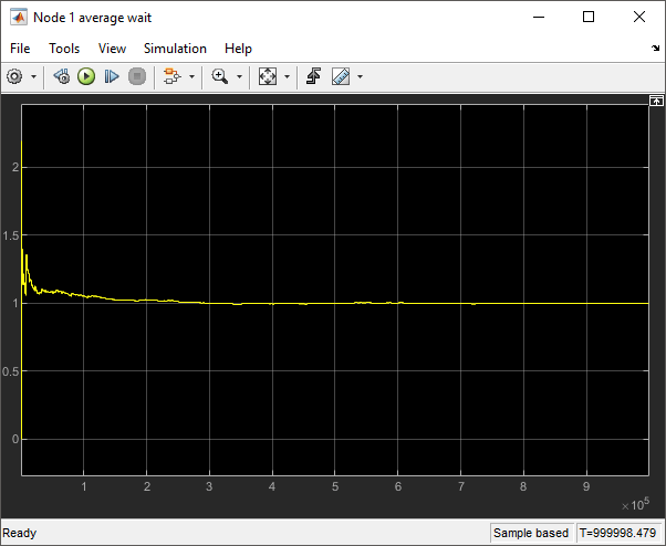
Simulate the model and observe that the mean waiting time in each queue in the network matches the calculated theoretical results.
The waiting time for the queue in node
1converges to1.
The waiting time for the queue in node
2converges to0.11.

The waiting time for the queue in node
3converges to0.88.

The waiting time for the queue in node
4converges to0.58.
References
[1] Jackson, James R. Operations research Vol. 5, No. 4 (Aug., 1957), pp 518-521.