Model RF Filter Using Circuit Envelope
This example shows how to model an RF filter using Circuit Envelope Library. In this example, you compare the input and output signal amplitudes to study the signal attenuation.
Model Overview
This example uses an LC bandpass filter designed to have a bandwidth of 200 MHz. The filter uses a three tone input signal to demonstrate the filter attenuation property for in-band and out-band frequencies. The input signal tones are:
700 MHz – Center frequency of the filter passband
600 MHz – Lower edge frequency of the filter passband
900 MHz – Frequency outside the filter passband
Define Model Variables and Settings
Define model variables for blocks that share parameter values using the InitFcn.
In Simulink® editor, select MODELING > SETUP > Model Settings >
Model Properties.In the
Model Propertiesdialog box, on the Callbacks tab in Model callbacks pane, selectInitFcn.In the Model initialization function pane, enter:
amp = ones(1,3); freq = [600 700 900]*1e6; stepsize = 1/500e6;Click OK.
In the Simulink tool bar, set the simulation stop time to
0.In Simulink editor, select MODELING > SETUP > Model Settings >
Model Settings Ctrl+EIn Configuration Parameters dialog box, set Solver to
discrete (no continuous states)and in Data Import/Export pane, clearSingle simulation output.
Required Blocks
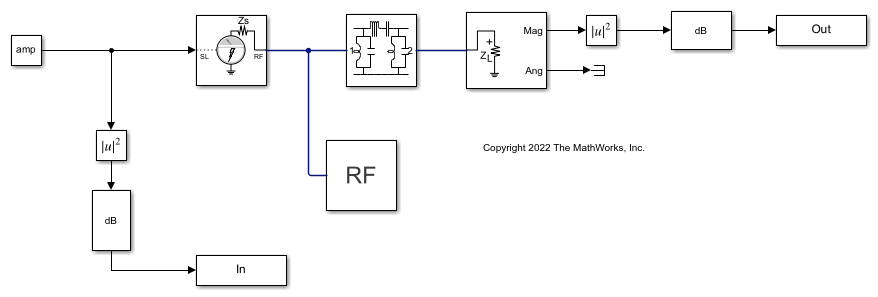
The filter system consists of LC Ladder, Inport, Outport, and Configuration blocks. The physical part of the model uses bidirectional RF signals. The blocks used in the system are:
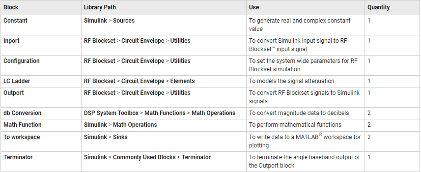
Connect the blocks as shown in the model or open the model attached in this example.
open_system("rffilter_ce.slx")
Configure Input Signal
Generate the three-tone input signal using these blocks:
Constant block specifies the amplitude of the signal.
Inport block configures the frequencies of the three tones.
Configuration block specifies the step size.
In the Constant block:
Set the Constant value to
amp, as defined in theInitFcn.
In the Inport block:
Set Source type to
Power.Set Carrier frequencies to
freq, as defined inInitFcn. Thefreqvariable sets the frequency of the three tones to 600 MHz, 700 MHz, and 900 MHz, respectively.Click OK.
In the Configuration block:
Set Step size to
stepsize, as defined inInitFcn.Clear Simulate noise.
Click OK.
The fundamental tones and harmonics are updated automatically when you run the model.
Configure RF Filter
In the LC Ladder block:
Set Ladder topology to
LC Bandpass Pi.Click Apply and then click OK.
Configure Output Settings
In the Outport block:
Set Sensor type to
Power.Set Output to
Magnitude and Angle Baseband.Set Carrier frequencies to
freq, as defined inInitFcn.Click OK.
Configure Other Blocks
In the Simulink editor, connect the
Angport of the Outport block to Terminator block to terminate the angle baseband output.In Math Function and Math Function 1 blocks, set Function to
magnitude^2and click OK. The block squares the magnitude of the input and output signal.In dB Conversion and dB Conversion 1 blocks, set Input Signal to
Powerand click OK. The block converts the input and output signals to dB.In To Workspace, change the Variable name to
In. In To Workspace 1, change the Variable name toOut. In both blocks, set Save format to Array and click OK.
Run Model
Select Simulation > Run to run the model.
sim("rffilter_ce.slx")
Plot and Analyze Attenuated Output Signals
Display the input and output signals using semilogx function, in dB.
Transfer the input and output dB values to the MATLAB® workspace using To Workspace block.
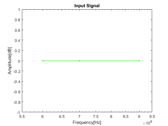
To view the input signal to RF Filter, plot
Inarray from the MATLAB workspace.
figure
h = semilogx(freq, In,'-gs','LineWidth',1,'MarkerSize',3,'MarkerFaceColor','r');
xlim([5.5e8,9.5e8]);
xlabel('Frequency[Hz]');
ylabel('Amplitude[dB]');
title('Input Signal');
To view the output signal (filtered attenuated signal), plot Out array from the MATLAB workspace.
figure
h1 = semilogx(freq, Out,'-gs','LineWidth',1,'MarkerSize',3,'MarkerFaceColor','r');
xlim([5.5e8,9.5e8]);
ylim([-25,1]);
xlabel('Frequency[Hz]');
ylabel('Amplitude[dB]');
title('Attenuated Output Signal');
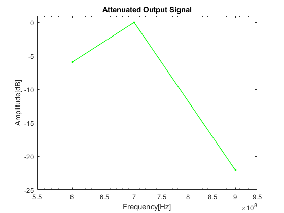
Compare the input and output signal plots to verify the attenuation caused by the filter. Notice that the RF filter does not attenuate the signal at the center frequency of 700 MHz.
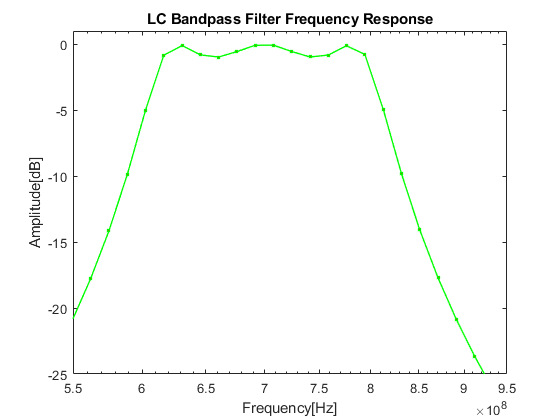
Analyze LC Bandpass Filter Response
Plot more points to better understand the response of the LC bandpass filter. Change the defined variables in Model Properties to: amp = ones(1,201); freq = logspace (8,10,201); stepsize = 1/500e6;.
Run the model. Notice that the signal is not attenuated within the 200 MHz range of the LC bandpass filter. Alternatively, you can run rffilter_ce3.slx. Note that rffilter_ce3.slx is loaded with the updated defined variables.
sim("rffilter_ce3.slx")
Plot the LC bandpass filter frequency response.
figure
h3 = semilogx(freq, Out,'-gs','LineWidth',1,'MarkerSize',3,'MarkerFaceColor','r');
xlim([5.5e8,9.5e8]);
ylim([-25,1]);
xlabel('Frequency[Hz]');
ylabel('Amplitude[dB]');
title('LC Bandpass Filter Frequency Response');