RLCG Transmission Line

Model RLCG transmission line

Libraries:
RF Blockset / Equivalent Baseband / Transmission Lines

Description

The RLCG Transmission Line block models the RLCG transmission line described in the block dialog box in terms of its frequency-dependent resistance, inductance, capacitance, and conductance. The transmission line, which can be lossy or lossless, is treated as a two-port linear network.

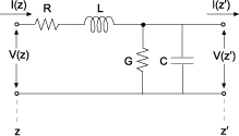
Cross-section of RLGC transmission line

where z′ = z + Δz.

To learn how you can use RLCG Transmission Line block to create baseband equivalent model, see Create Complex Baseband-Equivalent Model.

Parameters

expand all

Main

Resistance per length (ohms/m) — Resistance of RLGC transmission lines
`0` (default) | scalar

Resistance of the RLGC transmission lines, specified as a scalar in ohms/meters.

Inductance per length (H/m) — Inductance of RLGC transmission lines
`0` (default) | scalar

Inductance of the RLGC transmission lines, specified as a scalar in henries/meters.

Capacitance per length (F/m) — Capacitance of RLGC transmission lines
`0` (default)

Capacitance of the RLGC transmission lines, specified as a scalar in farad/meters

Conductance per length(S/m) — Conductance of RLGC transmission lines
`0` (default) | scalar

Conductance of the RLGC transmission lines, specified as a scalar in siemens per meter.

Frequency (Hz) — Frequency at which RLGC transmission line operate
`1e-9` (default)

Vector of frequency values at which the resistance, inductance, capacitance, and conductance values are known.

Interpolation method — Method to interpolate network parameters
`Linear` (default) | `Spline` | `Cubic`

Method to interpolate the network parameters, specified as one of the following:

Method	Description
`Linear`	Linear interpolation
`Spline`	Cubic spline interpolation
`Cubic`	Piecewise cubic Hermite interpolation

Transmission line length (m) — Physical length of transmission line
`0.01` (default) | scalar

Physical length of the transmission line, specified as a scalar in meters.

Stub mode — Type of stub
`Not a stub` (default) | `Shunt` | `Series`

The block enables you to model the transmission line as a stub or as a stubless line.

Stubless transmission Line

Not a stub—Not a stub
If you model a coaxial transmission line as stubless line, the Coaxial Transmission Line block first calculates the ABCD-parameters at each frequency contained in the modeling frequencies vector. It then uses the abcd2s function to convert the ABCD-parameters to S-parameters. For more information, see Stub Mode - Not a Stub.

Shunt Transmission Line

Shunt—This parameter provides a two-port network that consists of a stub transmission line that you can terminate with either a short circuit or an open circuit as shown in these diagrams.
Z_in is the input impedance of the shunt circuit. The ABCD-parameters for the shunt stub are calculated as
$\begin{matrix} A = 1 \\ B = 0 \\ C = 1 / Z_{i n} \\ D = 1 \end{matrix}$

Series Transmission Line

Series—This mode parameter provides a two-port network that consists of a series transmission line that you can terminate with either a short circuit or an open circuit as show in these diagrams.
Z_in is the input impedance of the series circuit. The ABCD-parameters for the series stub are calculated as
$\begin{matrix} A = 1 \\ B = Z_{i n} \\ C = 0 \\ D = 1 \end{matrix}$

Termination of stub — Stub termination
`Open` (default) | `Short`

Stub termination for stub modes Shunt and Series. Choices are Open or Short

Dependencies

To enable this parameter, select Shunt or Series in Stub mode

Visualization

Source of frequency data — Frequency data source
`User-specified` (default)

Frequency data source, specified as User-specified.

Frequency data (Hz) — Frequency data range
`[1e9:1e6:3e9]` (default) | vector

Frequency data range, specified as a vector in hertz.

Reference impedance (ohms) — Reference impedance
`50` (default) | nonnegative scalar

Reference impedance, specified as a nonnegative scalar in ohms.

Plot type — Type of data plot
`X-Y plane` (default) | `Composite data` | `Polar plane` | `Z Smith chart` | `Y Smith chart` | `ZY Smith chart`

Type of data plot to visualize using the given data, specified as one of the following:

X-Y plane — Generate a Cartesian plot of the data versus frequency. To create linear, semilog, or log-log plots, set the Y-axis scale and X-axis scale accordingly.
Composite data — Plot the composite data. For more information, see Create Plots Using Equivalent Baseband Library Blocks.
Polar plane — Generate a polar plot of the data. The block plots only the range of data corresponding to the specified frequencies.
Z smith chart, Y smith chart, and ZY smith chart — Generate a Smith^® chart. The block plots only the range of data corresponding to the specified frequencies.

Y parameter1 — Type of parameters to plot
`S11` (default) | `S12` | `S21` | `S22` | `GroupDelay` | `OIP3` | `IIP3` | `NF` | ...

Type of parameters to plot, specified as one of the following.

`S11`	`S12`	`S21`	`S22`
`GroupDelay`	`GammaIn`	`GammaOut`	`VSWRIn`
`VSWROut`	`OIP3`	`IIP3`	`NF`
`NFactor`	`NTemp`	`TF1`	`TF2`
`TF3`	`Gt`	`Ga`	`Gp`
`Gmag`	`Gmsg`	`GammaMS`	`GammaML`
`K`	`Delta`	`Mu`	`MuPrime`

Note

Y parameter1 is disabled when you select Plot type to Composite data.

Y parameter2 — Type of parameters to plot
`S11` (default) | `S12` | `S21` | `S22` | `GroupDelay` | `OIP3` | `IIP3` | `NF` | ...

Type of parameters to plot, specified as one of the following.

`S11`	`S12`	`S21`	`S22`
`GroupDelay`	`GammaIn`	`GammaOut`	`VSWRIn`
`VSWROut`	`OIP3`	`IIP3`	`NF`
`NFactor`	`NTemp`	`TF1`	`TF2`
`TF3`	`Gt`	`Ga`	`Gp`
`Gmag`	`Gmsg`	`GammaMS`	`GammaML`
`K`	`Delta`	`Mu`	`MuPrime`

Note

Y parameter2 is disabled when you select Plot type to Composite data.

Y format1 — Plot format
`Magnitude (decibels)` (default) | `Mag` | `Magnitude (linear)` | `Angle` | `Real` | `Imaginary` | ...

Plot format, specified as one of the following.

Y parameter1	Y format1
`S11`, `S12`, `S21`, `S22`, `GammaIn`, `GammaOut`, `TF1`, `TF2`, `TF3`, `GammaMS`, `GammaML`, and `Delta`.	`dB`, `Magnitude (decibels)`, `Abs`, `Mag`, `Magnitude (linear)`, `Angle`, `Angle(degrees)`, `Angle(radians)`, `Real`, `Imag`, and `Imaginary`.
`GroupDelay`	`ns`, `us`, `ms`, `s`, and `ps`.
`VSWRIn` and `VSWROut`.	`Magnitude (decibels)` and `None`.
`OIP3` and `IIP3`.	`dBm`, `W`, and `mW`.
`NF`	`dB` and `Magnitude (decibels)`.
`NFactor`, `K`, `Mu`, and `MuPrime`.	`None`
`NTemp`	`Kelvin`
`Gt`, `Ga`, `Gp`, `Gmag`, and `Gmsg`.	`dB`, `Magnitude (decibels)`, and `None`.

Dependencies

To enable Y format1, set Plot type to X-Y plane.

Y format2 — Plot format
`Magnitude (decibels)` (default) | `Mag` | `Magnitude (linear)` | `Angle` | `Real` | `Imaginary` | ...

Plot format, specified as one of the following.

Y parameter2	Y format2
`S11`, `S12`, `S21`, `S22`, `GammaIn`, `GammaOut`, `TF1`, `TF2`, `TF3`, `GammaMS`, `GammaML`, and `Delta`.	`dB`, `Magnitude (decibels)`, `Abs`, `Mag`, `Magnitude (linear)`, `Angle`, `Angle(degrees)`, `Angle(radians)`, `Real`, `Imag`, and `Imaginary`.
`GroupDelay`	`ns`, `us`, `ms`, `s`, and `ps`.
`VSWRIn` and `VSWROut`.	`Magnitude (decibels)` and `None`.
`OIP3` and `IIP3`.	`dBm`, `W`, and `mW`.
`NF`	`dB` and `Magnitude (decibels)`.
`NFactor`, `K`, `Mu`, and `MuPrime`.	`None`
`NTemp`	`Kelvin`
`Gt`, `Ga`, `Gp`, `Gmag`, and `Gmsg`.	`dB`, `Magnitude (decibels)`, and `None`.

Dependencies

To enable Y format2, set Plot type to X-Y plane.

X parameter — Frequency plot
`Freq` (default)

Frequency plot, specified as Freq.

X format — Frequency plot format
`Hz` (default) | `Auto` | `kHz` | `MHz` | `GHz` | `THz`

Frequency plot format, specified as one of the following.

`Auto`	`Hz`	`kHz`	`MHz`
`GHz`	`THz`

Y scale — Y-axis scale
`Linear` (default) | `Log`

Y-axis scale, specified as Linear or Log.

Dependencies

To enable this parameter, set Plot type to X-Y plane.

X scale — X-axis scale
`Linear` (default) | `Log`

X-axis scale, specified as Linear or Log.

Dependencies

To enable this parameter, set Plot type to X-Y plane.

Plot — Plot specified data
button

Plot the specified data using the plot button.

More About

expand all

Stub Mode - Not a Stub

This block calculates the ABCD-parameters using the physical length of the transmission line, d, and the complex propagation constant k using the equations:

$\begin{array}{l} A = \frac{e^{k d} + e^{- k d}}{2} \\ B = \frac{Z_{0} * (e^{k d} - e^{- k d})}{2} \\ C = \frac{e^{k d} - e^{- k d}}{2 * Z_{0}} \\ D = \frac{e^{k d} + e^{- k d}}{2} \end{array}$

Z₀ and k are vectors whose elements correspond to the elements of f, a vector of modeling frequencies, determined by the Output Port block. Both can be expressed in terms of the resistance (R), inductance (L), conductance (G), and capacitance (C) per unit length (meters)

$\begin{matrix} Z_{0} = \sqrt{\frac{R + j ω L}{G + j ω C}} \\ k = k_{r} + j k_{i} = \sqrt{(R + j ω L) (G + j ω C)} \end{matrix}$

where

$\begin{array}{l} R = \frac{1}{2 π σ_{c o n d} δ_{c o n d}} (\frac{1}{a} + \frac{1}{b}) \\ L = \frac{μ}{2 π} \ln (\frac{b}{a}) \\ G = \frac{2 π ω ε^{″}}{\ln (\frac{b}{a})} \\ C = \frac{2 π ε^{'}}{\ln (\frac{b}{a})} \end{array}$

In these equations:

a is the radius of the inner conductor.
b is the radius of the outer conductor.
σ_cond is the conductivity of the conductor.
μ is the permeability of the dielectric. μ = μ₀ μ_r, where:
- μ₀ is the permeability in free space.
- μ_r is the Relative permeability constant
The is a complex dielectric constant given by ε = ε′ − јε″= ε′ (1 − јtanδ)
ε′ is the real part of complex dielectric constant ε, ε′ = ε₀ε_r.
ε″ is the imaginary part of complex dielectric constant ε, ε″ = ε₀ε_rtan δ where :
- ε₀ is the permittivity of free space.
- ε_r is the Relative permittivity constant parameter value.
- tan δ is the Loss tangent of dielectric parameter value.
δ_cond is the skin depth of the conductor, which the block calculates as $1 / \sqrt{π f μ σ_{c o n d}}$ .

References

[1] Pozar, David M. Microwave Engineering. Hobken, NJ, John Wiley & Sons, Inc., 2005.

Version History

Introduced in R2009a

RLCG Transmission Line

Description

Parameters

Main

Resistance per length (ohms/m) — Resistance of RLGC transmission lines 0 (default) | scalar

Inductance per length (H/m) — Inductance of RLGC transmission lines 0 (default) | scalar

Capacitance per length (F/m) — Capacitance of RLGC transmission lines 0 (default)

Conductance per length(S/m) — Conductance of RLGC transmission lines 0 (default) | scalar

Frequency (Hz) — Frequency at which RLGC transmission line operate 1e-9 (default)

Interpolation method — Method to interpolate network parameters Linear (default) | Spline | Cubic

Transmission line length (m) — Physical length of transmission line 0.01 (default) | scalar

Stub mode — Type of stub Not a stub (default) | Shunt | Series

Stubless transmission Line

Shunt Transmission Line

Series Transmission Line

Termination of stub — Stub termination Open (default) | Short

Dependencies

Visualization

Source of frequency data — Frequency data source User-specified (default)

Frequency data (Hz) — Frequency data range [1e9:1e6:3e9] (default) | vector

Reference impedance (ohms) — Reference impedance 50 (default) | nonnegative scalar

Plot type — Type of data plot X-Y plane (default) | Composite data | Polar plane | Z Smith chart | Y Smith chart | ZY Smith chart

Y parameter1 — Type of parameters to plot S11 (default) | S12 | S21 | S22 | GroupDelay | OIP3 | IIP3 | NF | ...

Y parameter2 — Type of parameters to plot S11 (default) | S12 | S21 | S22 | GroupDelay | OIP3 | IIP3 | NF | ...

Y format1 — Plot format Magnitude (decibels) (default) | Mag | Magnitude (linear) | Angle | Real | Imaginary | ...

Dependencies

Y format2 — Plot format Magnitude (decibels) (default) | Mag | Magnitude (linear) | Angle | Real | Imaginary | ...

Dependencies

X parameter — Frequency plot Freq (default)

X format — Frequency plot format Hz (default) | Auto | kHz | MHz | GHz | THz

Y scale — Y-axis scale Linear (default) | Log

Dependencies

X scale — X-axis scale Linear (default) | Log

Dependencies

Plot — Plot specified data button

More About

Stub Mode - Not a Stub

References

Version History

See Also

Topics

Resistance per length (ohms/m) — Resistance of RLGC transmission lines
`0` (default) | scalar

Inductance per length (H/m) — Inductance of RLGC transmission lines
`0` (default) | scalar

Capacitance per length (F/m) — Capacitance of RLGC transmission lines
`0` (default)

Conductance per length(S/m) — Conductance of RLGC transmission lines
`0` (default) | scalar

Frequency (Hz) — Frequency at which RLGC transmission line operate
`1e-9` (default)

Interpolation method — Method to interpolate network parameters
`Linear` (default) | `Spline` | `Cubic`

Transmission line length (m) — Physical length of transmission line
`0.01` (default) | scalar

Stub mode — Type of stub
`Not a stub` (default) | `Shunt` | `Series`

Termination of stub — Stub termination
`Open` (default) | `Short`

Source of frequency data — Frequency data source
`User-specified` (default)

Frequency data (Hz) — Frequency data range
`[1e9:1e6:3e9]` (default) | vector

Reference impedance (ohms) — Reference impedance
`50` (default) | nonnegative scalar

Plot type — Type of data plot
`X-Y plane` (default) | `Composite data` | `Polar plane` | `Z Smith chart` | `Y Smith chart` | `ZY Smith chart`

Y parameter1 — Type of parameters to plot
`S11` (default) | `S12` | `S21` | `S22` | `GroupDelay` | `OIP3` | `IIP3` | `NF` | ...

Y parameter2 — Type of parameters to plot
`S11` (default) | `S12` | `S21` | `S22` | `GroupDelay` | `OIP3` | `IIP3` | `NF` | ...

Y format1 — Plot format
`Magnitude (decibels)` (default) | `Mag` | `Magnitude (linear)` | `Angle` | `Real` | `Imaginary` | ...

Y format2 — Plot format
`Magnitude (decibels)` (default) | `Mag` | `Magnitude (linear)` | `Angle` | `Real` | `Imaginary` | ...

X parameter — Frequency plot
`Freq` (default)

X format — Frequency plot format
`Hz` (default) | `Auto` | `kHz` | `MHz` | `GHz` | `THz`

Y scale — Y-axis scale
`Linear` (default) | `Log`

X scale — X-axis scale
`Linear` (default) | `Log`

Plot — Plot specified data
button