Analysis of Frequency Response of RF System
This example uses a few techniques to calculate the steady-state frequency response for a filter-based RF system built from RF Blockset™ Circuit Envelope library blocks. The first technique performs static analysis (harmonic balance) on a circuit comprising of inductors and capacitors. The second technique does time domain simulation using a similar circuit built with the Filter library block. The third technique facilitates small-signal analysis to obtain the frequency response of a filtering system that exhibits nonlinearity at a given operation point. This example helps you validate a circuit envelope model using a static analysis in the frequency domain, a time domain simulation, and small signal analysis in cases where the system exhibits non-linearity.
Frequency Domain Analysis
model = 'simrfV2_ac_analysis';
open_system(model);

The system consists of:
A Continuous Wave source and a series resistor to model a voltage source with internal source impedance.
Inductor and Capacitor blocks configured to model a third-order Chebyshev filter with a center frequency of 2.4 GHz.
An Outport block configured as a voltage sensor to measure the voltage across a load resistor.
A Configuration block, which sets up the circuit envelope simulation environment. As the system is linear, the harmonic balance analysis is done with a single simulation frequency and corresponds to an AC analysis.
Type
open_system('simrfV2_ac_analysis')at the Command Window prompt.Double-click the block labeled 'Specify Frequency Values' to provide a vector of frequencies.
Double-click the block labeled 'Calculate Frequency Response' to execute a script,
simrfV2_ac_analysis_callback, that analyzes the model at the specified frequencies and plots the response.
simrfV2_ac_analysis_callback([model '/Subsystem'], 'OpenFcn');

To configure a model with circuit envelope library blocks for harmonic balance:
In the Model Configuration parameters dialog box, set the Stop time parameter to zero.
Use a Continuous Wave block to drive the system.
Set the Carrier frequencies parameter in the Continuous Wave, Outport blocks, and the Fundamental Tones parameter in the Configuration block to the same vector of frequencies.
Close the open model
bdclose(model)
Time Domain Simulation
model = 'simrfV2_ac_analysis_tf';
open_system(model)

The system consists of:
A Random source generator that outputs a continuous random signal.
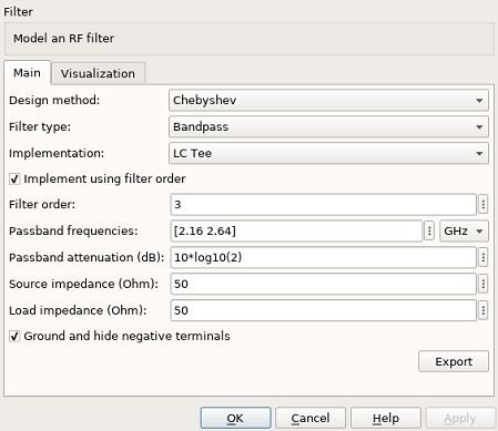
A Chebyshev filter constructed using the Filter library block and designed with a center frequency of 2.4 GHz and a bandwidth of 480 MHz.
Discrete Transfer Function Estimator block to view the frequency domain output of a time domain simulation.
Spectrum Analyzer to view the output.
View the filter designed parameters used in the Filter block mask.

View the implemented filter under the Filter block mask.
open_system([model '/Filter'],'force')

Simulate the transfer system model.
sim(model,5e-5)

Compare the outputs of the first and second model.
bdclose(model)
Small Signal Analysis
model = 'simrfV2_ac_analysis_ss';
open_system(model)

The system consists of:
A Random source generator that outputs a continuous random signal that is subsequently attenuated to ensure small signal input.
A constant source added to the random source to determine the non-linear operation point. Both signals are centered at 2.4 GHz.
An RF System comprising two elements; A saw filter constructed using the S-parameter library block with a center frequency of 2.45 GHz and a bandwidth of 112 MHz and an amplifier with 20dB of available power gain and non-linearity described by a 3rd-order intercept point of 30dBm.
Discrete Transfer Function Estimator block to view the frequency domain output of a time domain simulation measured over the 2.4 GHz carrier.
Spectrum Analyzer to view the output and compare it to saved output data.
Since the transient signal is small while the operation point is determined based on carrier-constant large signals, it is possible to use the transient small-signal approximation. In this approximation, non-linear interaction between transient signals is ignored, however the non-linear interaction between carrier-constant signals and its effect on the small signals is captured accurately. The small signal analysis is enabled in the advanced tab of the Configuration block mask.

Using small signal analysis, a subset of the full set of carriers used for steady state solution can be chosen for transient simulation. In this example, only the 2.4 GHz is of interest for transient analysis. Reducing the number of simulated carriers, accelerates the simulation. In this case, the small signal simulation is more than 15 times faster than a full non-linear circuit-envelope based simulation. Comparing the small-signal simulation results with those of a full circuit envelope simulation loaded from a file, it is evident that the results are practically identical.
sim(model)

Decreasing the operation point power in the constant block from 0.5 Watt down to zero, the system becomes effectively linear. A comparison between the curves illustrates the effect of the non-linearity on the transfer function. These effects include a decrease in overall amplitude due to compression and a widening of the filter profile at the lower-frequency side. The widening can be explained as the result of the cubic term in the amplifier polynomial response folding the original RF frequency of 2.4 GHz back onto itself, but with a frequency response that is flipped around its central frequency since 2.4 GHz is reached by reflection from -2.4 GHz. Since the Saw filter is centered at 2.45GHz, the flipped frequency response is centered at 2.35GHz. Summing the linear and cube terms effects yields a widened profile.

bdclose(model)
References
Ludwig, Reinhold and Pavel Bretchko, RF Circuit Design: Theory and Applications. Prentice-Hall, 2000.
Mass A. Stephen, Nonlinear Microwave and RF Circuits. Artech House, 2003.
See Also
Compare Time and Frequency Domain Simulation Options for S-parameters