Compare Time and Frequency Domain Simulation Options for S-parameters
This example shows how to use two different options for modeling S-parameters with the RF Blockset™ Circuit Envelope library. The Time-domain (rational) technique creates an analytical rational model that approximates the whole range of the data. This is a preferable technique when a good fit could be achieved with a small number of poles. When the data has a lot of details or high level of noise, this model becomes large and slow to simulate.
The frequency-domain technique is based on convolution, where the baseband impulse response depends on the simulation time step and the carrier frequency.
System Architecture
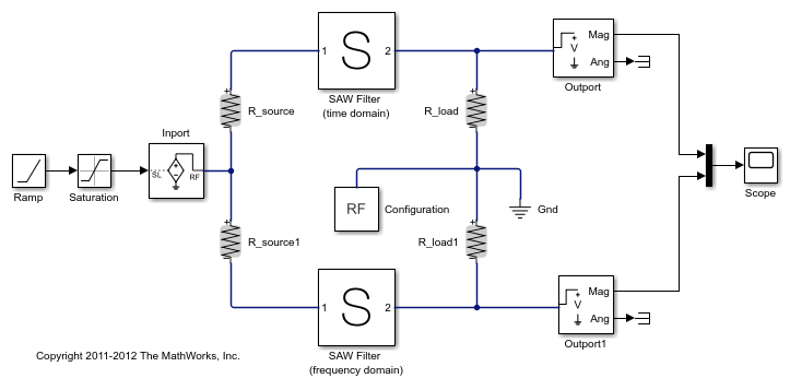
The system consists of:
An input envelope signal modeled with Simulink® blocks. The input signal is a ramp that goes from 0 to 1 in
TF_RAMP_TIME; the initial value ofTF_RAMP_TIMEis set to1e-6s. The carrier frequency of the signal isTF_FREQ; the initial value ofTF_FREQis set to2.4e9Hz.Two SAW filters, modeled by two S-parameter blocks using the same data file,
sawfilter.s2p. The block labeledSAW Filter (time domain)has its Modeling options parameter in the Modeling tab set toTime domain (rational). The block labeledSAW Filter (frequency domain)has its Modeling options parameter in the Modeling tab set toFrequency domainand the Automatically estimate impulse response duration is checked.A Scope block that displays the outputs of the two S-parameter blocks.
model = 'simrfV2_sparam_t_vs_f';
open_system(model);

Run Simulation with the Default Settings
Type
open_system('simrfV2_sparam_t_vs_f')at the Command Window prompt.Select Simulation > Run.
The outputs from both methods are very close to each other. The frequency-domain model (purple curve) captures the transfer function (steady-state value) a bit better.
scope = [model '/Scope'];
open_system(scope);
set_param(scope, 'YMax','0.45');
set_param(scope, 'YMin','0');
set_param(scope, 'TimeRange',num2str(1.01*TF_END_TIME));
sim(model);

Run the Simulation with the Very Steep Ramp
In the previous simulation, the rise time of the envelope TF_RAMP_TIME = 1e-6 was many orders of magnitude greater than the period of the carrier signal T = 1/TF_FREQ = 4.1667e-10. In other words, the envelope was much slower than the carrier. As the ramp time approaches the period of the carrier, the corresponding time effects are better captured by the time-domain model (yellow curve).
TF_RAMP_TIME = 1e-9;
TF_END_TIME = 1e-7;
set_param(scope, 'TimeRange',num2str(1.01*TF_END_TIME));
sim(model);
open_system(scope);

The result of the frequency-domain simulation can be improved by decreasing the time step of the simulation and manually setting the impulse duration time.
To continue the example:
Type
TF_STEP = 5e-10;at the Command Window prompt.Uncheck Automatically estimate impulse response duration in the modeling pane of
Saw filter (frequency domain)block and specify the Impulse Response Duration as1e-7.Select Simulation > Run.
TF_STEP = 5e-10;
sparam_freq  = [model '/SAW Filter  (frequency domain)'];
set_param(sparam_freq, 'AutoImpulseLength', 'off');
set_param(sparam_freq, 'ImpulseLength', '1e-7');
sim(model);
open_system(scope);

Run Simulation with Different Frequency
Rational-function approximation is not exact. To see the approximation error, double-click the "SAW Filter (time domain)" block. Information about the approximation appears under "Rational fitting results" in the bottom of the dialog box 'Modeling' pane.
open_system([model sprintf('/SAW Filter (time domain)')]);
For more details, select 'Visualization' panel, and click the 'Plot' button.
The rational fit algorithm (dotted curve) does a very good job for the most of the frequencies. However, sometimes it does not capture the sharp changes of S-parameter data.
simrfV2_click_dialog_button('Block Parameters: SAW Filter (time domain)', 'PlotButton');

Conversely, the frequency-domain method exactly reproduces the steady-state behavior at all carrier frequencies (by definition). Running the simulation for TF_FREQ = 2.54e9 produces drastically different results between the two S-parameter methods.
To continue the example:
Type
TF_FREQ = 2.54e9; TF_RAMP_TIME = 1e-6; TF_STEP = 3e-9; TF_END_TIME = 2.5e-6;at the Command Window prompt.Select Simulation > Run.
In this case, the frequency-domain model provides a better approximation of the original data.
TF_STEP = 3e-9;
TF_RAMP_TIME = 1e-6;
TF_FREQ = 2.54e9;
TF_END_TIME = 2.5e-6;
set_param(scope, 'YMax','1e-3');
set_param(scope, 'TimeRange',num2str(1.01*TF_END_TIME));
sim(model);
open_system(scope);


Run Simulation with Impulse Duration Set to Zero.
There is a special case that could be very helpful in practice. When the "Impulse Response Duration" of the s-parameters block is set to zero, the history of the input is no longer taken into consideration. Still, the model captures the transfer function (steady-state value) correctly. This is a fast and reliable way to model the ideal devices when the transient effects could be ignored.
To continue the example:
Specify the
Impulse Response DurationofSaw filter (frequency domain)block as0.Select Simulation > Run.
set_param(sparam_freq, 'ImpulseLength', '0');
sim(model);
open_system(scope);

Conclusion
In most practical RF systems, time- and frequency-domain techniques give similar answers. The time-domain method better captures the time-domain effects of the fast-changing envelopes, but relies on a rational fit approximation of the original data. The frequency-domain method is sensitive to the simulation time step; this option is recommended when the time-domain model does not provide a good fit.
close gcf;
bdclose(model);
clear model scope;
See Also
S-Parameters | Configuration | Inport | Outport