Transmission Lines, Delay-Based and Lumped Models

Open Script

This example shows how to simulate delay-based and lumped-element Transmission Line using blocks in the RF Blockset™ Circuit Envelope library. The example is sequenced to examine circuit envelope and passband differences, delay-based lossy transmission line sectioning, and lumped element implementation of delay.

System Architecture for Lossless Delay-Based Transmission Line

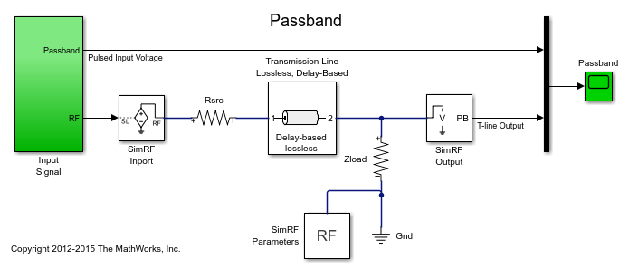
In this section, two RF Blockset™ models, simrf_xline_pb and simrf_xline_ce, illustrate lossless delay-based transmission line effects and the computational benefit of circuit envelope techniques.

model_pb = 'simrf_xline_pb';
model_ce = 'simrf_xline_ce';
load_system(model_ce)
open_system(model_pb)

The model, simrf_xline_pb, represents a passband signal as:

$I(t) \cos{2\pi f_c t} - Q(t) \sin{2\pi f_c t}$

The input is a pulse-modulated sinusoidal passband signal. For this particular case, I(t) equals zero, and Q(t) is the pulse modulation. The carrier frequencies are set to zero in the RF Blockset Inport and Outport blocks.

open_system([model_pb '/Input Signal']);

The circuit envelope model, simrf_xline_ce, represents an envelope signal as:

$$I(t) + j Q(t)$$

Again, I(t) equals zero, and Q(t) is the pulse modulation, but the carrier signal is not specified as part of the input signal. To model the carrier, the Carrier Frequencies parameter is set to $f_c$ in the RF Blockset Inport and Outport blocks.

open_system([model_ce '/Input Signal']);

Removal of the explicit sinusoidal carrier in the circuit-envelope model allows the simulation to reduce time-steps relative to the passband model.

Running the Lossless Delay-Based Transmission Line

Type open_system('simrf_xline_pb') or open_system('simrf_xline_ce') at the Command Window prompt.
Select Simulation > Run.

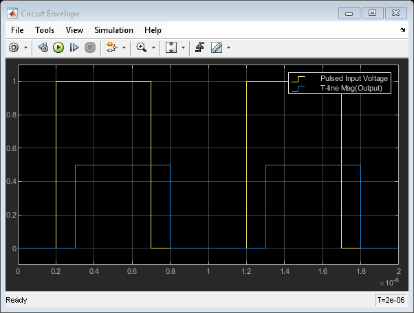
After simulating, the transmission delay is observable in a plot of input and output signals.

open_system([model_ce '/Circuit Envelope']);
sim(model_ce);

The carriers in modulated waveforms appear in passband signals, but only the modulation envelopes appear in circuit-envelope signals. Passband signals can be reconstructed from circuit envelope signals as:

$Re((I(t) + j Q(t)) e^{j2\pi f_c t})$

However, reconstruction of the passband signal this way requires additional time steps for the carrier.

sim(model_pb);
hline = plot(SPB_Data(:,1),SPB_Data(:,2),SCE_Data(:,1),SCE_Data(:,2),'--');
legend('Passband', 'Circuit Envelope')
title('Input Passband and Circuit Envelope Signals')
xlabel('Time')
ylabel('Voltage')
ylim([-1.1 1.1])

haxis = get(hline(1),'Parent');
plot(haxis,SPB_Data(:,1),SPB_Data(:,3),SCE_Data(:,1),SCE_Data(:,3),'--')
legend('Passband', 'Circuit Envelope')
title('Output of Passband and Circuit Envelope Signals')
xlabel('Time')
ylabel('Voltage')
ylim([-.55 .55])

Partitioning Delay-Based Lossy Transmission Lines

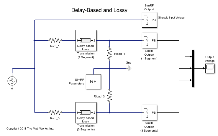
A conventional method for modeling distributed lossy transmission lines employs N two-port segments in cascade. Each segment consists of an ideal lossless delay line and resistance, where the segment delay equals the total line delay divided by N and the segment resistance equals the total line resistance divided by N. As the number of segments increases, the lumped model will more accurately represent the distributed system. This methodology requires a compromise between simulation time and model accuracy for increasing N. In RF Blockset, the Number of segments, the Resistance per unit length and the Line length are specified as dialog box parameters in the transmission line block.

model_seg = 'simrf_xline_seg';
open_system(model_seg)

System Architecture for Lossy Delay-Based Transmission Line

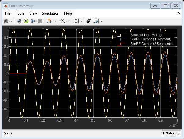
The lossy delay-based transmission line model, simrf_xline_seg, consists of two parallel arms excited by a RF Blockset sinusoidal source. The top arm employs a single segment transmission line, while the bottom arm uses a line consisting of 3 segments. The source and load resistances are not equal to the characteristic impedance of the transmission line. These differences affect the shape of the output response. For example, the output response will be overdamped when the source and load resistances are less than the characteristic impedance.

open_system([model_seg '/Output Voltage']);
sim(model_seg);

Increasing the number of line segments in the bottom arm from three to four and comparing responses show that three segments suffice for this configuration.

close_system([model_seg '/Output Voltage']);
ST_Data3 = ST_Data;
set_param([model_seg '/Transmission (3 Segments)'],'NumSegments','4')
sim(model_seg);
plot(haxis, ST_Data3(:,1), ST_Data3(:,4), ST_Data(:,1), ST_Data(:,4), '--')
legend('3 Segments', '4 Segments')
title('Delay-Based Lossy Transmission Line Output Signals')
xlabel('Time')
ylabel('Voltage')

System Architecture for Lumped Element Transmission Line

Differences between the lumped element and delay-based transmission lines are now examined. Consider the model simrf_xline_ll, where the dialog box parameter Model_type is Delay-based and lossy for the top arm and Lumped parameter L-section for the other two arms. The Inductance per unit length and Capacitance per unit length parameters values for the L-section lines are similar to a 50 $\Omega$ coaxial cable. Basic first order approximations for these lines are $Z_0 = \sqrt{L/C}$ and $T_D = \sqrt{L*C} * Length.$

model_ll = 'simrf_xline_ll';
open_system(model_ll)

Running the Lumped Element Transmission Line

Type open_system('simrf_xline_ll') at the Command Window prompt.
Select Simulation > Run.

The following graph shows how the number of lumped element segments affects the output. Speed and accuracy must be balanced when using the lumped-element transmission line block.

open_system([model_ll '/Circuit Envelope Output Voltage 200MHz Carrier']);
sim(model_ll);

Cleaning Up

Close the model and remove workspace variables.

close(get(haxis,'Parent'))
clear haxis hline;
bdclose({model_pb model_ce model_seg model_ll});
clear SCE_Data SPB_Data ST_Data ST_Data3 SLL_Data;
clear model_pb model_ce model_seg model_ll;

References

Sussman-Fort and Hantgan, SPICE Implementation of Lossy Transmission Line and Schottky Diode Models. IEEE Transactions on Microwave Theory and Techniques, Vol. 36, No. 1, January 1988

True Kenneth M, Data Transmission Lines and Their Characteristics. Application Note 806, April 1992