End-to-End Modeling of a Full Communications Link Using RF Blockset Channel Block

Load Data and Show RF Budget Analysis of the Link

Initially, the central frequency for transmission is set to 27 GHz and the antennas used in the RF budget analysis are created and shown. To accelerate the example execution, pre-calculated antenna data and simulation results are saved in a file that is downloaded on first run of the example. If internet connection is not available or there is interest in new calculation and simulation, set the variable load_all_data to false. Alternatively, individual control of loading from file can be achieved by setting 'useFile=false' in relevant functions and by setting load variables throughout the example to false.

%#ok<*ASGLU>
%#ok<*UNRCH>
CF = 27e9; % [Hz]
load_all_data = true;
[patch_1_tx,patch_1_rx] = createAntennas(CF,useFile=load_all_data);

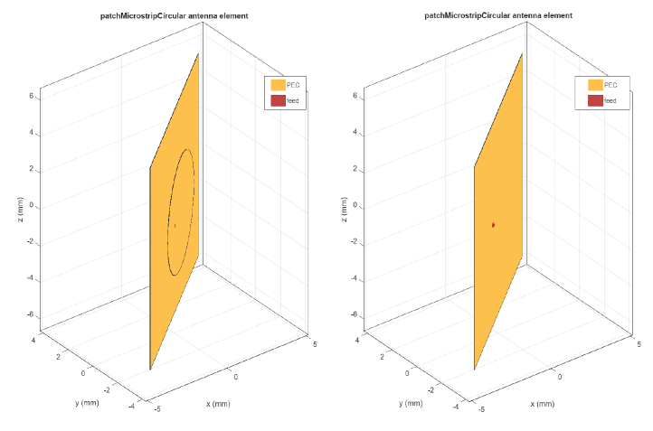
Show TX antenna and RX antennas by using the commands show(patch_1_tx) and show(patch_1_rx) respectively:

Load pre-created rfbudget object

load('budgetDesign.mat','rfb');

Type show(rfb) command at the command line to visualize the chain in the RF Budget Analyzer app.

The RF budget Analyzer App displays the RF Budget that in this case includes both a transmitter and a receiver, as well as a TransmitReceive Antenna element. This element represents both TX and RX antennas as well as a simple Free-Space medium between them represented as Path Loss. The angles used for the direction of departure and arrival are obtained from the propagation scenario shown below. Note that 326.5 degrees in transmitter elevation is 360-33.5=-33.5 degrees. The available input power at input to the transmitter is -30dBm.

Create rfsystem Object and Channel

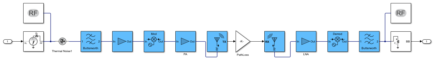
The rfbudget object is exported as an rfsystem System Object™ based on an RF Blockset CE model where the path loss in the medium between the antennas is modeled using a Simulink Gain block.

rfs=rfsystem(rfb);
open_system(rfs);
set_param(rfs.ModelName,'ZoomFactor','FitSystem')
[viewer,bsSite,ueSite,pm] = CreateChannel(patch_1_tx,patch_1_rx);

The CreateChannel helper function accepts two antennas as arguments. These are placed in the txSite and rxSite objects that are created and used below in the Channel block.

Change rfsystem Model to Include a Channel Block

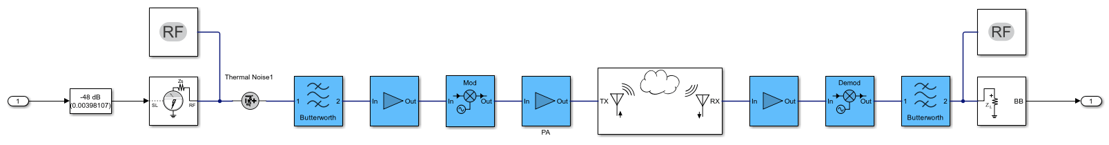
To obtain a higher fidelity model of propagation between the antennas, they, together with the Gain block representing the medium, are replaced with a Channel block. This is done by replacing the model internal to the rfsystem object with a pre-saved model named 'TXRX_1patch_NL'. In addition, some properties are defined such as input RF frequency, mixing LO frequency, output RF frequency transmitted by the antennas, as well as the simulation time step.

% Replace model in rfsystem
warnStruct = warning('off','Simulink:Engine:MdlFileShadowing');
origWarnStatus = warnStruct.state;
rfs.ModelName = 'TXRX_1patch_NL';
bdclose(rfs.ModelName);
% Set up simulation parameters
Fin = 4e9; % [Hz]
Flo = CF - Fin; % [Hz]
Fout = CF; % [Hz]
overSample = 4; % Over sample ratio
Tstep = 1/122.88e6/4/overSample; % Simulation sample rate: 1024*120KHz*4*overSample [s]
rfs.SampleTime = Tstep;
open_system(rfs);
set_param([rfs.ModelName '/Configuration1'],'StepSize','Tstep');
set_param([rfs.ModelName '/Configuration2'],'StepSize','Tstep');

Channel Block Mask Dialog and Propagation Scenario

The Channel block mask parameters are set to the outputs of the CreateChannel helper function. The first parameter, viewer, is the siteviewer object connected to building data in the OpenStreetMap file 'hongkong.osm' [1].

open_system([rfs.ModelName '/Channel']);

The second mask parameter is the Propagation model, pm that contains choices for the model such as maximum number of reflections accounted for (MaxNumReflections). Also, the Tx and Rx site mask parameters contain the txsite and rxsite objects bsSite and ueSite, created in the CreateChannel helper function and contain properties of the sites such as their geographic location and the antennas. Pressing the View Site button opens the siteviewer showing the scenario that is modeled:

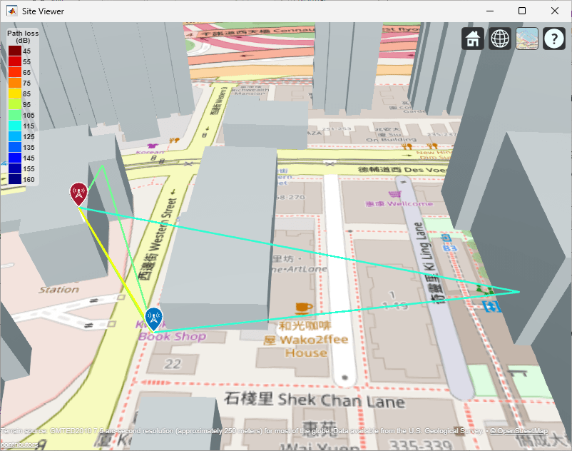
Note that the propagation scenario contains four rays, of which the dominant ones are the line-of-sight (LOS) ray (shown in yellow) and the ray reflected from the street (shown in green) that is just under the LOS ray in the viewer image. The other two rays are less dominant since the path loss associated with them is much larger. The ray angles can be obtained by pressing the ray in the siteviewer window.

Setup for 5G 3GPP Waveform Input

The rfsystem is fed by a New Radio test signal using FR2 bandwidth and Test Model 3.1 with 120KHz of subcarrier spacing for a total bandwidth of 400MHz. The following script creates this test signal. Such as a script can be obtained also using Export MATLAB script using the Wireless Waveform Generator app.

rc = "NR-FR2-TM3.1"; % Reference channel
bw = "400MHz"; % Channel bandwidth
scs = "120kHz"; % Subcarrier spacing
dm = "TDD"; % Duplexing mode
fprintf('Reference Channel = %s\n', rc);

tmwavegen = hNRReferenceWaveformGenerator(rc,bw,scs,dm,1);
tmwavegen = makeConfigWritable(tmwavegen);
tmwavegen.Config.SampleRate = 1/Tstep;
tmwavegen.Config.NumSubframes = 1;

[inWaveform,tmwaveinfo,resourcesinfo] = generateWaveform(tmwavegen, ...
    tmwavegen.Config.NumSubframes);

SampleRate = tmwaveinfo.Info.SamplingRate; % waveform sample rate
inWaveform=inWaveform./max(abs(inWaveform));

% Find waveform average power and normalizing factor:
PowMet = powermeter("ReferenceLoad", 1, ...
    "WindowLength", length(inWaveform), ...
    'Measurement','All');
[AvgPow, ~, PAPR] = PowMet(inWaveform);
release(PowMet);
G = -30-AvgPow(end);
disp(['Input power = ' num2str(AvgPow(end)+G), 'dBm']);
disp(['PAPR in = ' num2str(PAPR(end)), 'dB']);

Reference Channel = NR-FR2-TM3.1
Input power = -30dBm
PAPR in = 11.9864dB

Note that in the last part of the code above, the test signal created is normalized using a normalization factor G. The factor G is used in the following models to assure that the input power is -30dBm.

Show Input 5G Waveform in Spectrum and Calculate ACPR and EVM:

Show the spectrum of the input 5G waveform by invoking the Spectrum Analyzer. Use the normalization factor, G, to show expected input power.

% Setup and show Spectrum Analyzer:
SpectAnalyzer = spectrumAnalyzer;
SpectAnalyzer = setSpectAnalyzerProperties(SpectAnalyzer,Tstep,...
    {'Measurement'});
SpectAnalyzer(inWaveform*10^(G/20));

Calculate baseline ACPR and EVM values for input waveform using local helper functions found at the end of the example:

% Setup and perform ACPR measurement:
setupAndCalcACPR(SpectAnalyzer);
% Setup and perform EVM measurement:
setAndCalcEVM(tmwavegen,inWaveform,false);

ACPR data Adj = -43.3894 -43.8254
EVM RMS = 2.3757e-14%

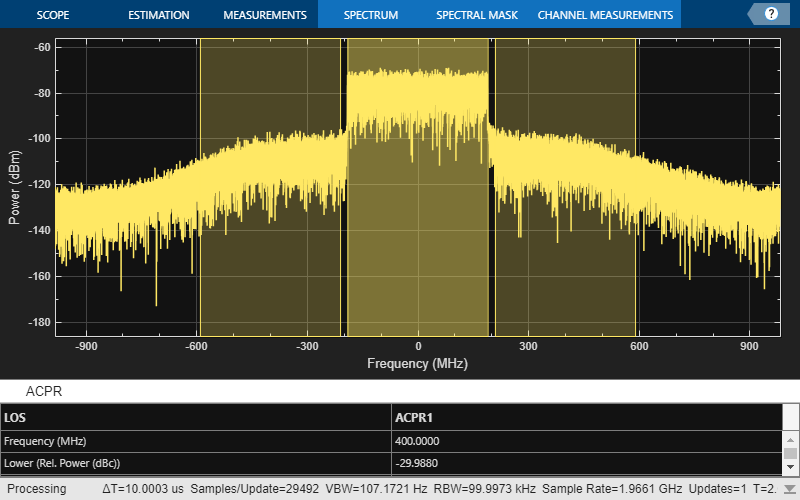
Simulate System for the Case of Line-of-Sight (LOS) Propagation:

The output results for the LOS case are obtained by sending the input waveform as signal to the rfsystem model described above. To accelerate the example run time, all the following simulations are preceded by a flag that indicates whether to load pre-saved simulation results or run the simulation. Change the load variable value to false to run the simulation. Note also that for viewing the spectrum of the output signal, it is enough to send the first 40000 signal samples into the RF system. Also, since the TX and RX sites are far, the temporal delay accumulated is too large for the time estimation process done in EVM calculations performed later in the example. This problem is solved by removing 175 time-samples from the output of all simulations to reduce the delay to values amenable to time estimation.

% Disallow reflections:
pm.MaxNumReflections=0;
% Simulate the rfsystem with part of the input waveform:
load_LOS_data = load_all_data;
if ~load_LOS_data
    largeDelay = 175; % large delay removal
    outWaveform_LOS = rfs([inWaveform(1:40000); zeros(largeDelay,1)]);
    outWaveform_LOS = outWaveform_LOS(1+largeDelay:end);
    release(rfs);
    save('TX1RX1ChanData3p1_LOS.mat','outWaveform_LOS');
else
    load('TX1RX1ChanData3p1_LOS.mat','outWaveform_LOS');
end
% Measure power output waveform
PowMet.WindowLength = length(outWaveform_LOS);
[AvgPow, ~, PAPR] = PowMet(outWaveform_LOS);
release(PowMet);
disp(['Output power = ' num2str(AvgPow(end)), 'dBm']);
disp(['Output PAPR = ' num2str(PAPR(end)), 'dB']);
% Setup and show Spectrum Analyzer:
SpectAnalyzer = spectrumAnalyzer;
SpectAnalyzer = setSpectAnalyzerProperties(SpectAnalyzer,Tstep,{'LOS'});
SpectAnalyzer(outWaveform_LOS);
% Setup and perform ACPR measurement:
setupAndCalcACPR(SpectAnalyzer);

Output power = -41.115dBm
Output PAPR = 10.4108dB
ACPR data Adj = -29.988 -29.1783

Simulate System for Multi-Path Propagation:

The output results for the multi-path case are obtained by sending the input waveform as signal to the same rfsystem model used above, with channel block propagation model changed to allow reflection.

% Allow one reflection:
pm.MaxNumReflections=1;
% Simulate the rfsystem with part of the input waveform:
load_1st_ref_data = load_all_data;
if ~load_1st_ref_data
    largeDelay = 175; % large delay removal
    outWaveform_1st_ref = rfs([inWaveform(1:40000); zeros(largeDelay,1)]);
    outWaveform_1st_ref = outWaveform_1st_ref(1+largeDelay:end);
    release(rfs);
    save('TX1RX1ChanData3p1_1st_ref.mat','outWaveform_1st_ref');
else
    load('TX1RX1ChanData3p1_1st_ref.mat','outWaveform_1st_ref');
end
% Measure power output waveform
[AvgPow, ~, PAPR] = PowMet(outWaveform_1st_ref);
release(PowMet);
disp(['Output power = ' num2str(AvgPow(end)), 'dBm']);
disp(['Output PAPR = ' num2str(PAPR(end)), 'dB']);
% Setup and show Spectrum Analyzer:
SpectAnalyzer = spectrumAnalyzer;
SpectAnalyzer = setSpectAnalyzerProperties(SpectAnalyzer,Tstep,...
    {'LOS','LOS + 1st reflections'});
SpectAnalyzer([outWaveform_LOS outWaveform_1st_ref]);
% Setup and perform ACPR measurement:
setupAndCalcACPR(SpectAnalyzer);

Output power = -40.3495dBm
Output PAPR = 10.2786dB
ACPR data Adj = -29.988 -29.1783

Introducing reflections into the channel model results in multipath fading artifacts with dips in spectrum due to cancelation between signals traversing the two dominant paths.

Change rfsystem Model to Include an 8-element TX Array and Simulate

To model a system with an 8-element transmitter array, initially the antenna array itself is created.

% Create 8-element TX antenna array
[patch_1_tx,patch_1_rx,patch_8_array_tx] = createAntennas(CF,useFile=load_all_data);

Use show(patch_8_array_tx) to show TX antenna array

Next, an 8-way splitter that splits the input signal into each of the RF chains is designed and its S-parameter data is obtained.

% Create S-parameter data for 8-output Wilkinson splitter
swc_wb = createSplitterData(CF,useFile=load_all_data);

Set useFile to false in order to recalculate data and show splitter. Note that design and calculation of the splitter is available in RF PCB Toolbox.

The model is replaced with a model containing 8 RF chains, each with a phase shift to tilt array 33.5 degrees from broadside in elevation. The array is positioned vertically and therefore the beam can only be steered along the elevation direction. Note that the calculation of the phase shifts relies on functionality available in Phased Array System Toolbox.

% Calculate phase shifts
phaseShifts = CreatePhaseShifts(CF,90-33.5);
% Change rfsystem model to include array
rfs.ModelName = 'TXRX_8patch_NL';
bdclose(rfs.ModelName);
open_system(rfs);
set_param([rfs.ModelName '/Configuration1'],'StepSize','Tstep');
% Create channel with an 8-element patch array in TX system
[~,bsSiteArray,ueSite,pm] = CreateChannel(patch_8_array_tx,patch_1_rx,viewer);
pm.MaxNumReflections=1;

The subsystem TX system contains the splitter and 8 chains. Each chain is identical to the single chain simulated before except for the added phase shift block.

open_system([rfs.ModelName '/TX system'],'force');

As before, the output results for the 8-element TX array case are obtained by sending the input waveform as signal to the corresponding rfsystem model.

load_array_data = load_all_data;
if ~load_array_data
    largeDelay = 175; % large delay removal
    outWaveform_array_1st_ref = rfs([inWaveform(1:40000); zeros(largeDelay,1)]);
    outWaveform_array_1st_ref = outWaveform_array_1st_ref(1+largeDelay:end);
    release(rfs);
    save('TX8RX1ChanData3p1_1st_ref.mat','outWaveform_array_1st_ref');
else
    load('TX8RX1ChanData3p1_1st_ref.mat','outWaveform_array_1st_ref');
end
% Measure power output waveform
[AvgPow, ~, PAPR] = PowMet(outWaveform_array_1st_ref);
release(PowMet);
disp(['Output power = ' num2str(AvgPow(end)), 'dBm']);
disp(['Output PAPR = ' num2str(PAPR(end)), 'dB']);
% Setup and show Spectrum Analyzer:
SpectAnalyzer = spectrumAnalyzer;
SpectAnalyzer = setSpectAnalyzerProperties(SpectAnalyzer,Tstep,...
    {'Single element','Array'});
SpectAnalyzer([outWaveform_1st_ref outWaveform_array_1st_ref]);
% Setup and perform ACPR measurement:
setupAndCalcACPR(SpectAnalyzer);

Output power = -30.5282dBm
Output PAPR = 10.5461dB
ACPR data Adj = -30.7643 -30.0149

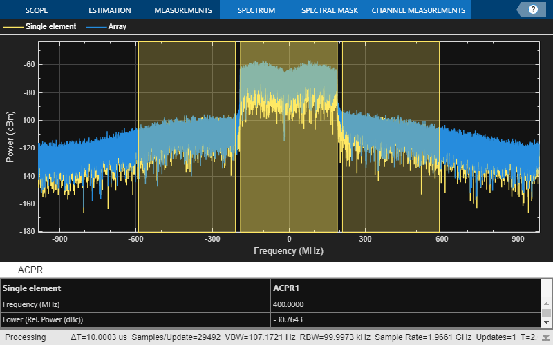
Comparing the spectrum for scenarios with single-element and 8-element TX systems, the latter shows higher received power since the signal is radiated towards the RX antenna with higher directivity.

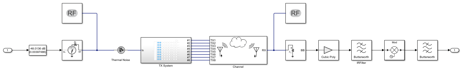
Use Accelerated Model to Simulate Entire 5G Frame for EVM Calculation

Up until now the simulation results were only processed to show the spectrum of the output signal, which required only a limited amount of samples. However, EVM calculation requires processing the entire 5G frame of 1ms, which translates into roughly 2 million samples. This results in a long simulation at the high-fidelity level provided by the full CE model used above. To accelerate the simulation, we consider that CE simulation becomes slow when there are many internal states in the system together with nonlinearity that requires Newton iteration at each simulation time step. A significant portion of the internal states in the system is due to the large S-parameter representation of the splitter and antennas. A much faster simulation can be achieved if the nonlinearity can be separated from the splitter and antenna models. This separation can be done by noting that the initial amplifier in each RF chain is followed by a mixer with 50 ohm input impedance. This means that the S22 and S12 terms of the S-parameter representation of the amplifier are not affecting the simulation and the amplifier can be decomposed into reflection effects governed by S11 and unidirectional frequency-dependent gain with nonlinearity effects governed by S21 and OIP3. The latter can be modeled using the RF Idealized Baseband library that, while limited in its ability to represent any system at high fidelity, is much faster than CE. At the end of the RF chain, the PA amplifier has a constant 50 ohm output impedance and is unidirectional. This implies that it too could be modeled within RF Idealized Baseband library and the mismatch at the antenna ports modeled using CE. The new model is placed in the rfsystem object and shown below. It can be seen within the TX system that for each RF chain, the nonlinear portion (including the initial amplifier, mixer, and PA) is replaced by fast RF Idealized Baseband blocks. Note that the initial amplifier block is replaced by a linear CE block containing only S11 created by zeroing all other S-parameter terms (CMD240withNF_cut_only_s11.s2p), an Idealized Baseband nonlinear amplifier described by OIP3 and frequency-independent gain extracted at 4GHz, and an Idealized Baseband S-Parameters block including all terms except S11, with S21 normalized to the gain extracted at 4GHz (CMD240withNF_cut_zero_s11_norm_at4GHz.s2p). Similarly, due to the unidirectionality of the LNA in the RX side, it and all following elements in that single chain can be replaced by fast RF Idealized Baseband blocks.

% Replace model in rfsystem for accelerated simulation:
rfs.ModelName = 'TXRX_8patch_NL_idealized';
bdclose(rfs.ModelName);
open_system(rfs);
set_param([rfs.ModelName '/Configuration1'],'StepSize','Tstep');
[~,bsSiteArray,ueSite,pm] = CreateChannel(patch_8_array_tx,patch_1_rx,viewer);
pm.MaxNumReflections=1;

% Show the subsystem TX system implemented using Idealized Baseband blocks:
open_system([rfs.ModelName '/TX System'],'force');

Next, simulate system for a TX with 8-element array for entire 5G frame.

load_array_data = load_all_data;
if ~load_array_data
    largeDelay = 175; % large delay removal
    % outWaveform_array_1st_ref_whole = rfs([inWaveform; zeros(largeDelay,1)]);
    outWaveform_array_1st_ref_whole = rfs([inWaveform(1:40000); zeros(largeDelay,1)]);
    outWaveform_array_1st_ref_whole = outWaveform_array_1st_ref_whole(1+largeDelay:end);
    release(rfs);
    save('AntObjsAndReceived5GSignals.mat',...
        'outWaveform_array_1st_ref_whole','-append');
else
    load('AntObjsAndReceived5GSignals.mat',...
        'outWaveform_array_1st_ref_whole');
end
% Measure power output waveform
PowMet.WindowLength = length(outWaveform_array_1st_ref_whole);
[AvgPow, ~, PAPR] = PowMet(outWaveform_array_1st_ref_whole);
release(PowMet);
disp(['Output power = ' num2str(AvgPow(end)), 'dBm']);
disp(['Output PAPR = ' num2str(PAPR(end)), 'dB']);

Output power = -30.7279dBm
Output PAPR = 11.6511dB

For comparison purposes, simulate system for TX system with 1-element array for entire 5G frame.

load_array_data = load_all_data;
if ~load_array_data
    rfs.ModelName = 'TXRX_1patch_NL_idealized';
    bdclose(rfs.ModelName);
    open_system(rfs);
    set_param([rfs.ModelName '/Configuration1'],'StepSize','Tstep');
    largeDelay = 175; % large delay removal
    outWaveform_1st_ref_whole = rfs([inWaveform; zeros(largeDelay,1)]);
    outWaveform_1st_ref_whole = outWaveform_1st_ref_whole(1+largeDelay:end);
    release(rfs);
    save('AntObjsAndReceived5GSignals.mat','outWaveform_1st_ref_whole',...
        '-append');
else
    load('AntObjsAndReceived5GSignals.mat','outWaveform_1st_ref_whole');
end
% Setup and show Spectrum Analyzer:
SpectAnalyzer = spectrumAnalyzer;
SpectAnalyzer = setSpectAnalyzerProperties(SpectAnalyzer,Tstep,...
    {'Single element','Array'});
SpectAnalyzer([outWaveform_1st_ref_whole outWaveform_array_1st_ref_whole]);
% Setup and perform ACPR measurement:
setupAndCalcACPR(SpectAnalyzer);

ACPR data Adj = -29.9426 -29.8172

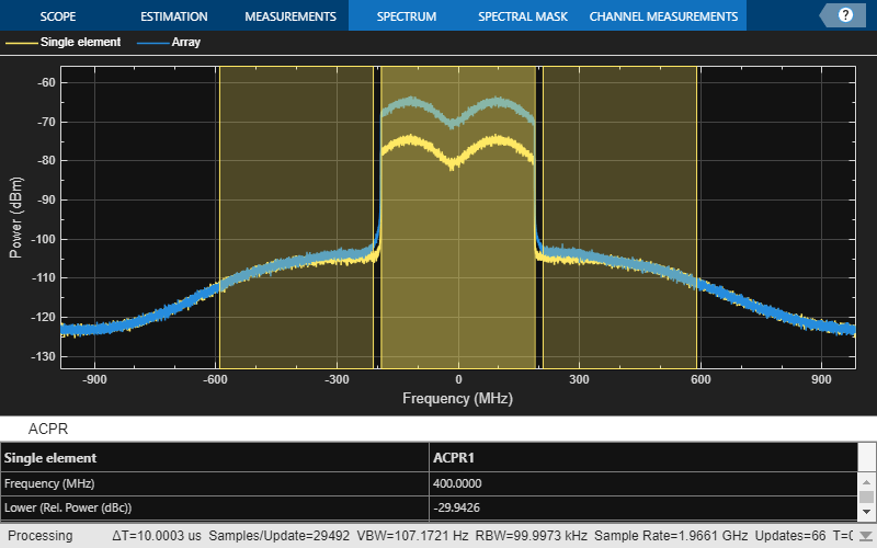
Notice that with the much longer simulated time period, the spectrum is averaged many more times and hence the effect of noise is less visible. With less visible noise effects, it becomes evident that while the array scenario yields higher received power across the band, the fading dips and peaks remain similar. This is since the array beam is not narrow enough to suppress the path reflecting from the street as that path is very close to the LOS path in its departing angle. The array curve is roughly 10dB above the single element curve in accordance with the improvement in antenna gain directed towards the LOS path. The simulation using Idealized Baseband blocks in the manner described above is faster than full CE simulation by a factor of roughly 9 and with little loss in simulation accuracy. Had the system had bidirectional elements throughout the RF chains or strong nonlinearity that requires balancing nonlinear multi-frequency interaction across elements, replacing CE with Idealized Baseband blocks would have resulted in significant loss in accuracy.

Finally, the results of simulating the entire 5G frame are used to study EVM performance of the systems. Initially for the single element case.

setAndCalcEVM(tmwavegen,outWaveform_1st_ref_whole,true)

EVM RMS = 4.4225%

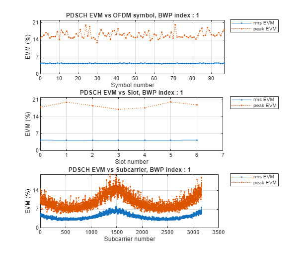
Note that the EVM peaks for subcarriers of the 5G signal that correspond to the frequency at which the spectrum exhibits a fading dip. For the LOS case, the EVM RMS is 4.27% with little variation over subcarrier index.

EVM is also measured for the 8-element TX system:

setAndCalcEVM(tmwavegen,outWaveform_array_1st_ref_whole,true)
warnStruct = warning(origWarnStatus,'Simulink:Engine:MdlFileShadowing');

EVM RMS = 1.4301%

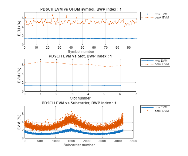
As expected, for the 8-element array, the EVM values are lower and correspondingly the constellations are denser around the ideal reference points. This is since, as was seen in the spectrum above, the 8-element array yields higher received power and improved output signal to noise ratio.

Close the open model:

bdclose(rfs.ModelName);

References

Local Functions

function SpectAnalyzer = setSpectAnalyzerProperties(SpectAnalyzer, Tstep, ChannelNames)
    % Setup properties for ACPR Calculation
    SpectAnalyzer.SampleRate = 1/Tstep;
    SpectAnalyzer.AveragingMethod = "running";
    SpectAnalyzer.SpectralAverages = 1024;
    SpectAnalyzer.ReferenceLoad = 1;
    SpectAnalyzer.RBWSource= "Property";
    SpectAnalyzer.RBW = 1e5;
    SpectAnalyzer.OverlapPercent = 0;
    SpectAnalyzer.ChannelMeasurements.Enabled = true;
    SpectAnalyzer.Method = "welch";
    SpectAnalyzer.AveragingMethod = "exponential";
    SpectAnalyzer.ForgettingFactor = 0.99;
    SpectAnalyzer.ChannelNames = ChannelNames;
end

function setupAndCalcACPR(SpectAnalyzer)
    % Setup properties for ACPR Calculation
    pause(5)
    SpectAnalyzer.MeasurementChannel = 1;
    SpectAnalyzer.ChannelMeasurements.Algorithm = 'ACPR';
    SpectAnalyzer.ChannelMeasurements.Span = 380.016e6;
    SpectAnalyzer.ChannelMeasurements.NumOffsets = 1;
    SpectAnalyzer.ChannelMeasurements.AdjacentBW = 380.016e6;
    SpectAnalyzer.ChannelMeasurements.ACPROffsets = 400e6;
    SpectAnalyzer.ChannelMeasurements.Enable = true;
    SpectAnalyzer.ChannelMeasurements.FilterShape='None';
    pause(5)
    % Compute and display ACPR measurements
    tmp = getMeasurementsData(SpectAnalyzer);
    ACPR_out(1) = tmp.ChannelMeasurements.ACPRLower(1);
    ACPR_out(2) = tmp.ChannelMeasurements.ACPRUpper(1);
    disp(['ACPR data Adj = ' num2str(ACPR_out(1)), ' ' num2str(ACPR_out(2))]);
end

function setAndCalcEVM(tmwavegen,waveform,plotEVM)
    % Setup properties for EVM calculation
    cfg = struct();
    cfg.Evm3GPP = false;
    cfg.TargetRNTIs = [];
    cfg.PlotEVM = plotEVM;
    cfg.DisplayEVM = false;
    cfg.Label = tmwavegen.ConfiguredModel{1};
    cfg.UseWholeGrid = true;
    cfg.TimeSyncEnable = true;
    cfg.CorrectCoarseFO = false;
    cfg.CorrectFineFO = true;
    cfg.PdcchEnable = false;
    % Compute and display EVM measurements
    [evmInfo,eqSym,refSym] = hNRDownlinkEVM(tmwavegen.Config,waveform,cfg);
    disp(['EVM RMS = ' num2str(evmInfo.PDSCH.OverallEVM.RMS*100) '%']);
end