Model RF Complex Baseband S-Parameters in Simulink

Open Script

This example shows you how to use the Idealized Baseband S-parameters block to model the RF complex baseband S-parameters in Simulink®. The example compares different solvers that you can use to model the RF complex baseband S-parameters in Simulink and in the circuit envelope domain. The Idealized Baseband S-parameters block allows you to design single-carrier perfectly matched RF systems, whereas the Circuit Envelope (CE) S-parameter block allows you to design multi-carrier RF systems with impedance mismatches.

System Architecture

This example uses of two systems. The first system compares fixed-step time-domain solvers, and the second system compares continuous time-domain solvers and frequency-domain solvers.

Fixed-step solvers include:

NDF2 — Balance narrowband and wideband accuracy. This solver is suitable for situations where the frequency content of the signals in the system is unknown relative to the Nyquist rate.
Trapezoidal — Perform narrowband simulations. Frequency warping and the lack of damping effects make this method unsuitable for most wideband simulations.
Backward Euler — Simulate the largest class of systems and signals. Damping effects make this solver suitable for wideband simulation, but overall accuracy for this solver is low.

Continuous solvers include:

ode15s – Solve stiff differential equations and DAEs using a variable order method
ode23s – Solve stiff differential equations using a low-order method
ode23t (trap) – Solve moderately stiff ODEs and DAEs using the trapezoidal rule
ode23tb (trap+BE) – Solve stiff differential equations using the trapezoidal rule and backward differentiation formula

Frequency-domain (digital filter) modeling uses a 1-D digital filter.

The systems also model and compare the S-parameters in the interpreted execution and code generation simulation modes.

Define Simulation Parameters

Define sample time, samples per frame, and carrier frequency as the simulation parameters.

sampleTime = 8e-6;
samplesPerFrame = 512;
carrierFrequency = 2.45e9;

Open and Run Fixed-Step Solver System

Open the fixed-step solver system.

open_system("idealsparams_fs.slx")

Run the fixed-step solver system.

sim("idealsparams_fs.slx");

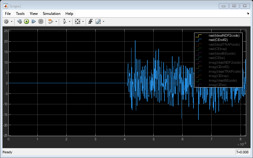
All solutions for a particular fixed-step time-domain solver are the same after the differences in the initialization time disappear. Compare the Ideal and CE S-parameter characteristics using the mask visualization tabs.

Open and Run Continuous Time Domain Solvers and Frequency Domain Solvers System

Open the continuous time-domain and frequency-domain modeling system.

open_system("idealsparams_ode.slx")

Run the continuous time-domain and frequency-domain modeling system.

sim("idealsparams_ode.slx");

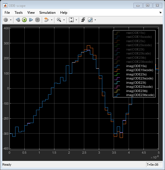
All solutions for a particular ODE solver are the same. But the solutions differ for the Ideal and CE frequency-domain solvers as they use different digital filter windowing schemes.