RF Receiver Modeling for LTE Reception

Model Description

An LTE waveform is generated, filtered, transmitted through a propagation channel and fed into an RF Blockset receiver model. The RF model can be assembled using commercially available parts. EVM measurements are performed on the RF receiver output.

This example is implemented using MATLAB® and Simulink®, which interact at runtime. The functional partition is as follows:

The measurement testbench is implemented with a MATLAB script using an RF System object as the device under test (DUT). LTE frames are streamed between testbench and DUT.

Generate LTE Waveform

In this section we generate the LTE waveform using the LTE Toolbox. We use the reference measurement channel (RMC) R.6 as defined in TS 36.101 [ 1 ]. This RMC specifies a 25 resource elements (REs) bandwidth, equivalent to 5 MHz. A 64 QAM modulation is used. All REs are allocated. Additionally, OCNG noise is enabled in unused REs.

Only one frame is generated. This frame will then be repeated a number of times to perform the EVM measurements.

% Configuration TS 36.101 25 REs (5 MHz), 64-QAM, full allocation
rmc = lteRMCDL('R.6');
rmc.OCNGPDSCHEnable = 'On';

% Create eNodeB transmission with fixed PDSCH data
rng(2) % Fixed random seed (arbitrary)
data = randi([0 1],sum(rmc.PDSCH.TrBlkSizes),1);

% Generate 1 frame, to be repeated to simulate a total of N frames
[tx,~,info] = lteRMCDLTool(rmc,data); % 1 frame

% Calculate the sampling period and the length of the frame
SamplePeriod = 1/info.SamplingRate;
FrameLength = length(tx);

Initialize Simulation Components

This section initializes some of the simulation components:

% Number of simulation frames N >= 1
N = 3;

% Preallocate vectors for results for N-1 frames
% Note: EVM is not measured in the first frame to avoid transient effects
evmpeak = zeros(N,1);
evmrms = zeros(N,1);

Design RF Receiver

The initial design of the RF receiver is done using the RF Budget Analyzer app. The receiver consists of a LNA, a direct conversion demodulator, and a final amplifier. All stages include noise and non-linearity.

load rfb.mat

Type show(rfb) to display the initial design of the RF receiver in the RF Budget Analyzer app.

Create RF model for simulation

From the RF budget object you can automatically create a model that can be used for circuit envelope simulation.

rfx = rfsystem(rfb);
rfx.SampleTime = SamplePeriod;
open_system(rfx)

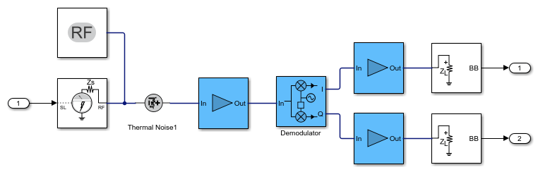
Extend the model of the RF receiver

You can modify the model created in the previous section to include additional RF impairments and components. You can modify the created RF Blocket model as long as you do not change the input / output ports. This section loads a modified Simulink model that performs the following functions:

You can open and inspect the modified model.

model = 'simrfV2_lte_receiver';
open_system(model)

Simulate Frames

This section simulates the specified number of frames. The RF system object simulates the Circuit Envelope model in Accelerator mode to decrease run time. After processing the first frame with the Simulink model, its state is preserved and automatically passed to the successive frame.

The output of the Simulink model is stored in the variable rx, which is available in the workspace. Any delays introduced to this signal are removed after performing synchronization. The EVM is measured on the resulting waveform.

load rfs.mat
EVMalg.EnablePlotting = 'Off';
cec.PilotAverage = 'TestEVM';

for n = 1:N
    [I,Q] = rfs(tx);
    rx = complex(I,Q);

    % Synchronize to received waveform
    if n == 1
        Offset = lteDLFrameOffset(rmc,squeeze(rx),'TestEVM');
    end

    % Compute and display EVM measurements
    evmmeas = simrfV2_lte_receiver_evm_cal(rmc,cec,squeeze(rx),EVMalg);
    evmpeak(n) = evmmeas.Peak;
    evmrms(n) = evmmeas.RMS;
end

Low edge EVM, subframe 0: 2.900%
High edge EVM, subframe 0: 2.895%
Low edge EVM, subframe 1: 2.804%
High edge EVM, subframe 1: 2.821%
Low edge EVM, subframe 2: 2.764%
High edge EVM, subframe 2: 2.768%
Low edge EVM, subframe 3: 2.796%
High edge EVM, subframe 3: 2.801%
Low edge EVM, subframe 4: 2.805%
High edge EVM, subframe 4: 2.813%
Low edge EVM, subframe 6: 2.812%
High edge EVM, subframe 6: 2.801%
Low edge EVM, subframe 7: 2.799%
High edge EVM, subframe 7: 2.787%
Low edge EVM, subframe 8: 2.785%
High edge EVM, subframe 8: 2.785%
Low edge EVM, subframe 9: 2.761%
High edge EVM, subframe 9: 2.766%
Averaged low edge EVM, frame 0: 2.802%
Averaged high edge EVM, frame 0: 2.803%
Averaged EVM frame 0: 2.803%
Averaged overall EVM: 2.803%
Low edge EVM, subframe 0: 2.801%
High edge EVM, subframe 0: 2.803%
Low edge EVM, subframe 1: 2.803%
High edge EVM, subframe 1: 2.808%
Low edge EVM, subframe 2: 2.776%
High edge EVM, subframe 2: 2.762%
Low edge EVM, subframe 3: 2.803%
High edge EVM, subframe 3: 2.803%
Low edge EVM, subframe 4: 2.780%
High edge EVM, subframe 4: 2.776%
Low edge EVM, subframe 6: 2.847%
High edge EVM, subframe 6: 2.867%
Low edge EVM, subframe 7: 2.820%
High edge EVM, subframe 7: 2.829%
Low edge EVM, subframe 8: 2.816%
High edge EVM, subframe 8: 2.824%
Low edge EVM, subframe 9: 2.901%
High edge EVM, subframe 9: 2.896%
Averaged low edge EVM, frame 0: 2.817%
Averaged high edge EVM, frame 0: 2.819%
Averaged EVM frame 0: 2.819%
Averaged overall EVM: 2.819%
Low edge EVM, subframe 0: 3.212%
High edge EVM, subframe 0: 3.189%
Low edge EVM, subframe 1: 3.001%
High edge EVM, subframe 1: 3.009%
Low edge EVM, subframe 2: 2.760%
High edge EVM, subframe 2: 2.776%
Low edge EVM, subframe 3: 2.809%
High edge EVM, subframe 3: 2.798%
Low edge EVM, subframe 4: 2.883%
High edge EVM, subframe 4: 2.877%
Low edge EVM, subframe 6: 2.936%
High edge EVM, subframe 6: 2.946%
Low edge EVM, subframe 7: 2.827%
High edge EVM, subframe 7: 2.826%
Low edge EVM, subframe 8: 2.776%
High edge EVM, subframe 8: 2.774%
Low edge EVM, subframe 9: 2.821%
High edge EVM, subframe 9: 2.828%
Averaged low edge EVM, frame 0: 2.890%
Averaged high edge EVM, frame 0: 2.889%
Averaged EVM frame 0: 2.890%
Averaged overall EVM: 2.890%

Visualize Measured EVM

This section plots the measured peak and RMS EVM for each simulated frame.

figure
plot((1:N),100*evmpeak,'o-')
title('EVM peak %')
xlabel('Number of frames')

figure
plot((1:N),100*evmrms,'o-')
title('EVM RMS %')
xlabel('Number of frames')

Cleaning Up

Close the Simulink model and remove the generated files.

release(rfs)
close_system(rfs,0)

Appendix

This example uses the following helper function:

Selected Bibliography