simulateFrequencyResponse
R2026bSimulate circuit in frequency domain and obtain real and imaginary impedance
Since R2025a
Syntax
Description
[
simulates the equivalent circuit model, realImpedance,imaginaryImpedance] = simulateFrequencyResponse(circuitModel,frequency)circuitModel, in the frequency
domain and returns the real and imaginary impedance.
[
also plots the frequency response and returns the handle to the plot. This plot is the
Nyquist representation of the circuit impedance.realImpedance,imaginaryImpedance,figureHandle] = simulateFrequencyResponse(circuitModel,frequency,Plot="on")
Examples
This example shows how to simulate two different electrochemical
impedance spectroscopy (EIS) models in the frequency domain by using the
simulateFrequencyResponse function.
Create a fractional-order equivalent circuit model with a resistor in series with a parallel configuration of a second resistor and a capacitor.
eisfom = eisModel("R0+(R1,C1)")eisfom =
EISModel with properties:
CircuitTopology: "R0+(R1,C1)"
NumParameters: 3
ParameterList: ["R0" "R1" "C1"]
ParameterValues: [0.0250 0.0035 150]
CircuitImpedance: "(R0 + ((R1 * (1/(i*w*C1))) / (R1 + (1/(i*w*C1)))))"
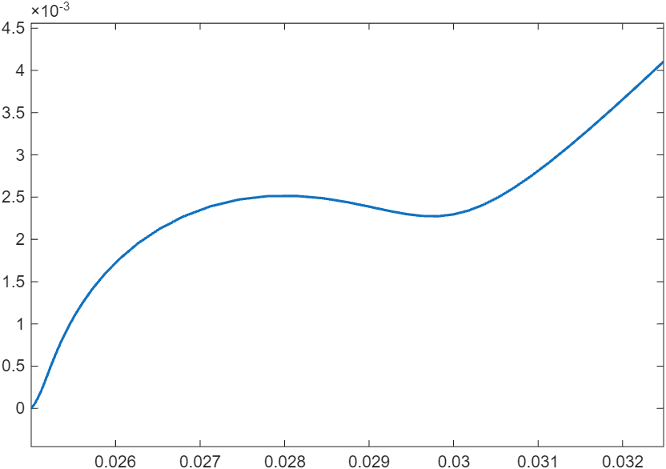
ParameterList: ["R0" "R1" "C1"]Define the frequency points you want to simulate the model at.
freq = logspace(-2,5,100)
Simulate the EIS circuit at these frequencies and plot the frequency response.
[simRealZ, simImagZ] = simulateFrequencyResponse(eisfom,freq);
plot(simRealZ,-simImagZ,linewidth=1.5)
axis equal
Now add a Warburg impedance term to the EIS circuit topology and observe how the frequency response changes.
eisfom.CircuitTopology = "R0 + (R1,C1) + SIW1";eisfom =
EISModel with properties:
CircuitTopology: "R0 + (R1,C1) + SIW1"
NumParameters: 4
ParameterList: ["R0" "R1" "C1" "SIW1"]
ParameterValues: [0.0250 0.0035 150 1.0000e-03]
CircuitImpedance: "((R0 + ((R1 * (1/(i*w*C1))) / (R1 + (1/(i*w*C1))))) + (SIW1*(w)^(-1/2) - SIW1*i*(w)^(-1/2)))"
ParameterList: ["R0" "R1" "C1" "SIW1"]Simulate the circuit and plot the frequency response. Starting in R2026b, you can
plot the frequency response directly by using the Plot name-value
argument of the simulateFrequencyResponse function.
[simRealZ,simImagZ,handle] = simulateFrequencyResponse(eisfom,freq,Plot="on");