Model Battery Temperatures Using Reduced-Order Thermal Models
This example shows how to derive and use a linear state‑space thermal model for a battery cell using the Partial Differential Equation Toolbox™ and integrate it into a Simscape™ network.
Deriving a reduced‑order model (ROM) directly from the energy‑conservation equations maintains physically meaningful thermal behavior of the battery cell and enables faster simulations. The full‑order thermal model, typically obtained through a finite‑volume or finite‑element discretization, captures heat transfer and thermal coupling across the cell by using a large set of algebraic and differential equations. Although accurate, these high‑dimensional models are often too computationally expensive for system‑level studies, hardware‑in‑the‑loop testing, or online estimation.
To reduce the model and preserves the underlying physics, you formulate the thermal dynamics in a state‑space form. By mapping the mass and conduction matrices from the energy‑balance equations to the E and A matrices of a descriptor state‑space system, the ROM preserves the correct heat‑capacity distribution and conductive pathways. This ensures that predicted temperatures, cooling responses, and thermal time constants remain consistent with the original discretized model.
Once you express the system in state‑space form, you can apply model‑reduction techniques to obtain a compact representation with far fewer states. The ROM maintains the dominant thermal dynamics, supports specified temperature measurement locations, and reproduces the effect of cooling on selected surfaces. At the same time, the compact size of the ROM allows simulations to run faster, making it suitable for real‑time applications and integration in larger Simscape system models.
Use Partial Differential Equation Toolbox to Perform Thermal Simulation
Before creating the ROM, use the Partial Differential Equation Toolbox to simulate the thermal behavior of the cell for comparison. In this example, you investigate the thermal behavior of a 21700 cylindrical cell with bottom cooling, ambient-exposed surfaces, and a uniform heat-generation rate throughout the cell volume. A 21700 cylindrical cell is a common lithium-ion battery cell format with standardized dimensions of 21 mm in diameter and 70 mm in length.
Import Cell Geometry
Import the cell geometry and define the temperature‑sensor locations along the side surface.
gm = importGeometry("CylindricalGeometry.stl");
model = femodel("AnalysisType","thermalTransient","Geometry",gm);
model = generateMesh(model,"Hmin",1E-5);
cellRadius = 0.0105;
cellLength =  0.0700;

%Cell top shoulder
shoulderNodeTop = findNodes(model.Mesh,"nearest",[cellRadius;0;cellLength]);
%Can surface 10 mm from the top
can10mmFromTop = findNodes(model.Mesh,"nearest",[cellRadius;0;cellLength-0.01]);
%Can surface midway point along the height
canMid = findNodes(model.Mesh,"nearest",[cellRadius;0;cellLength/2]);
%Can surface 10 mm from the bottom
can10mmFromBottom = findNodes(model.Mesh,"nearest",[cellRadius;0;0.01]);
%Cell bottom shoulder
shoulderNodeBottom = findNodes(model.Mesh,"nearest",[cellRadius;0;0]);
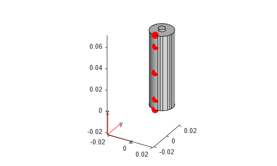
Display the cell geometry together with the temperature‑sensor points on the cell surface.
figure
title("Geometry with Probe Locations")
pdegplot(gm);
hold on;
plot3(model.Mesh.Nodes(1,shoulderNodeTop),model.Mesh.Nodes(2,shoulderNodeTop),model.Mesh.Nodes(3,shoulderNodeTop),'ro','MarkerSize',10,'MarkerFaceColor','r');
plot3(model.Mesh.Nodes(1,can10mmFromTop),model.Mesh.Nodes(2,can10mmFromTop),model.Mesh.Nodes(3,can10mmFromTop),'ro','MarkerSize',10,'MarkerFaceColor','r');
plot3(model.Mesh.Nodes(1,canMid),model.Mesh.Nodes(2,canMid),model.Mesh.Nodes(3,canMid),'ro','MarkerSize',10,'MarkerFaceColor','r');
plot3(model.Mesh.Nodes(1,can10mmFromBottom),model.Mesh.Nodes(2,can10mmFromBottom),model.Mesh.Nodes(3,can10mmFromBottom),'ro', 'MarkerSize',10,'MarkerFaceColor','r');
plot3(model.Mesh.Nodes(1,shoulderNodeBottom),model.Mesh.Nodes(2,shoulderNodeBottom),model.Mesh.Nodes(3,shoulderNodeBottom),'ro','MarkerSize',10,'MarkerFaceColor','r');
Specify Cell Geometry and Thermal Properties
For the thermal simulation of the battery, define the thermal properties of the cell.
thermalConductivity= [0.6; 0.6; 12]; % W/m-K
density = 2800; % Kg/m^3
heatCapacity = 850; %J/Kg-K
model.MaterialProperties = materialProperties("ThermalConductivity",thermalConductivity,"MassDensity",density,"SpecificHeat",heatCapacity);
thermalDiffusivity = thermalConductivity/(density*heatCapacity);
volume = cellLength*pi*cellRadius^2; % m^2
Define the simulation initial conditions, boundary conditions, and loads.
initialBatteryTemperature = 298; % K
simulationTime = 600; % s
heatGeneration = 5;% W
volumetricHeatGeneration = heatGeneration/volume; % W/m^3
ambientTemperature = 298; % K
bottomConvectionCoefficient = 200; % W/(m^2*K)
naturalConvectionCoefficient = 30; % W/(m^2*K)
Define Thermal Boundary Conditions
Define the thermal boundary conditions for the model. To represent cooling through the bottom plate, identify the bottom face of the cell and apply a convective face load.
cooledBottomFace = nearestFace(gm,[0,0,0]);
model.FaceLoad(cooledBottomFace) = faceLoad("ConvectionCoefficient",bottomConvectionCoefficient,...
    "AmbientTemperature",ambientTemperature);
All remaining external faces exchange heat with the ambient through convective cooling.
naturalConvectionFaces = setdiff(cellFaces(gm,1,"external"),cooledBottomFace);
model.FaceLoad(naturalConvectionFaces) = faceLoad("ConvectionCoefficient",naturalConvectionCoefficient,...
    "AmbientTemperature",ambientTemperature);
A constant volumetric heat load represents the heat generated during the charging and discharging of the cell.
model.CellLoad = cellLoad("Heat",volumetricHeatGeneration);Solve and Visualize Thermal Model
After you define the geometry, material properties, and boundary conditions, you can solve the thermal model by using the solve function of the Partial Differential Equation Toolbox.
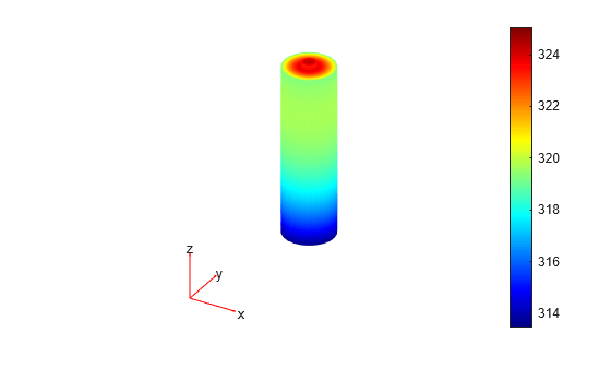
model.CellIC = cellIC("Temperature",initialBatteryTemperature);
Rt = solve(model,0:60:simulationTime);
figure
title("Temperature Profile of the Cell at Final Timestep")
pdeplot3D(model.Mesh,"ColorMapData",Rt.Temperature(:,end))
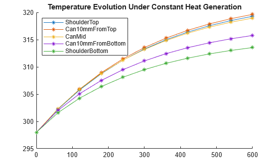
Finally, visualize the temperature response at the specified sensor locations.
hProbe = figure;
title("Temperature Evolution Under Constant Heat Generation")
hold on
plot(Rt.SolutionTimes,Rt.Temperature(shoulderNodeTop,:),"-*")
plot(Rt.SolutionTimes,Rt.Temperature(can10mmFromTop,:),"-*")
plot(Rt.SolutionTimes,Rt.Temperature(canMid,:),"-*")
plot(Rt.SolutionTimes,Rt.Temperature(can10mmFromBottom,:),"-*")
plot(Rt.SolutionTimes,Rt.Temperature(shoulderNodeBottom,:),"-*")
legend("ShoulderTop","Can10mmFromTop","CanMid","Can10mmFromBottom","ShoulderBottom","Location","northwest");
Reduce Model for Simscape
To generate a ROM and use it in Simscape, create a new model by using the femodel function in the Partial Differential Equation Toolbox. To create a model for modal thermal analysis, set the AnalysisType argument to thermalModal.
model = femodel("AnalysisType","thermalModal","Geometry",gm);
model = generateMesh(model,"Hmin",1E-5);
model.MaterialProperties = materialProperties("ThermalConductivity",thermalConductivity,...
    "MassDensity",density,"SpecificHeat",heatCapacity);
model.CellIC = cellIC("Temperature",initialBatteryTemperature);
Solve for modes of the thermal model in a specified decay range.
Rm = solve(model,'DecayRange',[-inf,0.05]);To generate the ROM, use the reduce function in the Partial Differential Equation Toolbox. Specify the modal analysis results obtained in the previous step.
rom = reduce(model,'ModalResults',Rm);Get the load matrix F which relates to the internal uniform heat generation.
model.CellLoad = cellLoad("Heat",1);
mats = assembleFEMatrices(model,"F");
F = mats.F;
Compute a separate G boundary matrix for each boundary condition. Each G matrix encodes how that boundary extracts heat proportional to the local temperature and augments the conductive operator so the overall decay rates reflect the specified cooling strength and location.
bottomBoundaryLoad = cooledSurface(model,cooledBottomFace);
naturalConvectionBoundaryLoad = cooledSurface(model,naturalConvectionFaces);
Get the nodes on the cooled sides.
bottomFaceNodes = findNodes(model.Mesh,'region', ...
    "Face",cooledBottomFace);

naturalConvectionFaceNodes = findNodes(model.Mesh,'region', ...
    "Face",naturalConvectionFaces);
Calculate State-Space Matrices
These equations define the generalized state‑space formulation:
where u denotes the inputs, y denotes the outputs, and x denotes the states. For the thermal model, the inputs u represent the heat transfer at the cell interfaces, while the outputs y correspond to the temperatures at the specified measurement locations.
The matrix D represents direct feedthrough from heat‑exchange inputs to temperature outputs, which typically does not occur in thermal systems. Therefore, you can neglect D and all elements are set to zero in this formulation.
You can extract the thermal mass matrix E, the thermal stiffness matrix A, and the initial state conditions directly from the reduced‑order model.
romParameters.ThermalStiffnessMatrix = -rom.K;
romParameters.ThermalMassMatrix = rom.M;
romParameters.InitialThermalState = rom.InitialConditions;
Then, determine the matrices B and C corresponding to the thermal interfaces and the temperature measurements. The thermal input matrix B and the thermal output matrix C are constructed separately for each interface to capture their individual contributions. For the temperature sensors located along the side of the cell, only the thermal output matrix C is required, incorporating all specified measurement positions.
romParameters.ProbeThermalOutputMatrix = rom.TransformationMatrix([shoulderNodeTop,can10mmFromTop,canMid,can10mmFromBottom,shoulderNodeBottom],:);
For each thermal interface (the cooling plate at the bottom, the ambient‑exposed surfaces, and the coupling to the electrical model), you must define the corresponding portion of the thermal input matrix B and the thermal output matrix C. These matrices expose the heat flow applied at each interface and the resulting temperature at that same interface.
At the interface with the cooling plate, the applied heat flow is assumed to be evenly distributed over the contact area. To obtain the interface temperature, you average the temperatures across that surface.
bottomArea = calculateFaceAreas(rom.Mesh,cooledBottomFace);
romInterfaceParameters.BottomArea = bottomArea;
romInterfaceParameters.BottomConvectionCoefficient = bottomConvectionCoefficient;
romInterfaceParameters.AmbientTemperature = ambientTemperature;
romParameters.BottomThermalInputMatrix = rom.TransformationMatrix' * bottomBoundaryLoad / bottomArea;
bottomAverageOperator = 1/numel(bottomFaceNodes) * ones(1,numel(bottomFaceNodes));
romParameters.BottomThermalOutputMatrix = bottomAverageOperator * rom.TransformationMatrix(bottomFaceNodes,:);
Apply the same approximations to the ambient‑cooled surfaces of the cell.
naturalConvectionArea = calculateFaceAreas(rom.Mesh,naturalConvectionFaces);
romInterfaceParameters.NaturalConvectionArea = naturalConvectionArea;
romInterfaceParameters.NaturalConvectionCoefficient = naturalConvectionCoefficient;
romParameters.NaturalConvectionThermalInputMatrix= rom.TransformationMatrix' * naturalConvectionBoundaryLoad / naturalConvectionArea;
naturalConvectionAverageOperator = 1/length(naturalConvectionFaceNodes) * ones(1,numel(naturalConvectionFaceNodes));
romParameters.NaturalConvectionThermalOutputMatrix = naturalConvectionAverageOperator * rom.TransformationMatrix(naturalConvectionFaceNodes,:);
The electrical model uses a lumped representation of the cell temperature, based on the average temperature across the entire volume. The model also assumes that the internally generated heat is uniformly distributed throughout the geometry.
cellVolume = model.Mesh.volume;
romParameters.CellThermalInputMatrix = rom.TransformationMatrix' * F / cellVolume;
cellAverageOperator = 1/width(model.Mesh.Nodes) * ones(1,width(model.Mesh.Nodes));
romParameters.CellThermalOutputMatrix = cellAverageOperator * rom.TransformationMatrix;
Validate ROM
Now integrate the resulting matrices into a custom Simscape block. This block exposes the thermal interfaces as thermal nodes. In this example, this block includes the required interface to the cell model and the optional interfaces for natural convection, as well as the cooling plate located at the bottom of the cell. To specify the total number of interfaces, use the Number of interfaces parameter. The block also provides a parameter for specifying the temperatures that you want to monitor.
To validate the ROM, a constant heat‑flow‑rate source models the heat that the battery cell generates. This heat matches the same heat‑flow‑rate input used in the partial differential equation model.
Open the model that includes the ROM block with the thermal interfaces, and use applyROMParametersToModelWorkspace to assign the calculated ROM parameters to the model workspace.
validationModelName = "thermalROMValidation";
open_system(validationModelName);
applyROMParametersToModelWorkspace(validationModelName,romParameters,romInterfaceParameters);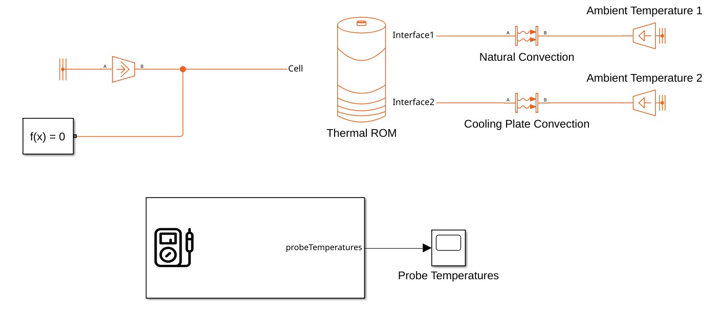
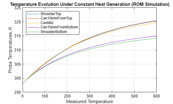
Simulate the model and plot the temperatures for the defined thermal sensors.
validationSimOut = sim(validationModelName);
validationSimOut.simlog.Thermal_ROM.probeTemperatures.plot;
xlabel("Measured Temperature")
ylabel("Probe Temperatures, K")
title("Temperature Evolution Under Constant Heat Generation (ROM Simulation)")
legend(["ShoulderTop","Can10mmFromTop","CanMid","Can10mmFromBottom","ShoulderBottom"],"Location","northwest")
grid on
Integrate Electrical Cell Model
To use the Thermal ROM block together with an electrical cell model, the electrical block must expose a scalar thermal node for coupling to the thermal model. The electrical block reads the temperature at this node to compute its electrical behavior and injects the corresponding heat generation back into the same thermal node.
Open the model that contains the ROM block thermally coupled to the electrical model and load the ROM parameters to the model workspace. The battery is discharged at 5 A for 300 s, then remains idle for the rest of the simulation.
cellModelName = "thermalROMCell";
open_system(cellModelName);
applyROMParametersToModelWorkspace(cellModelName,romParameters,romInterfaceParameters);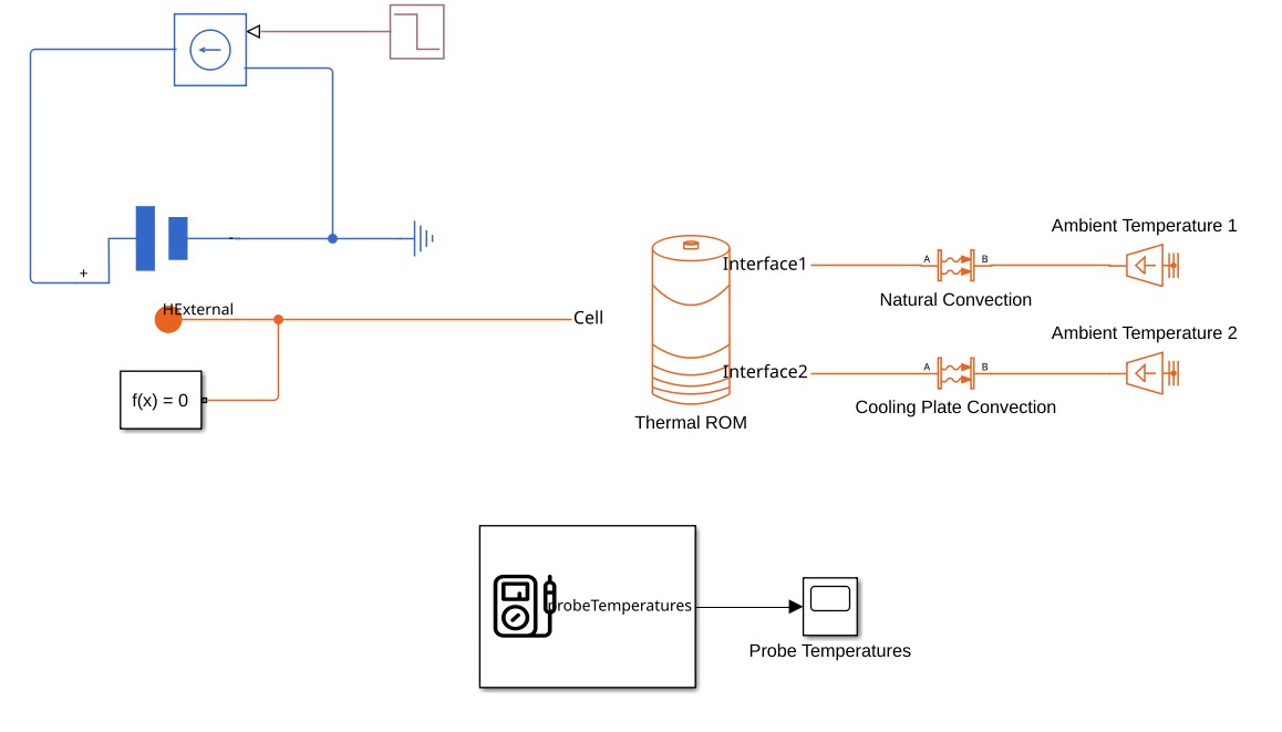
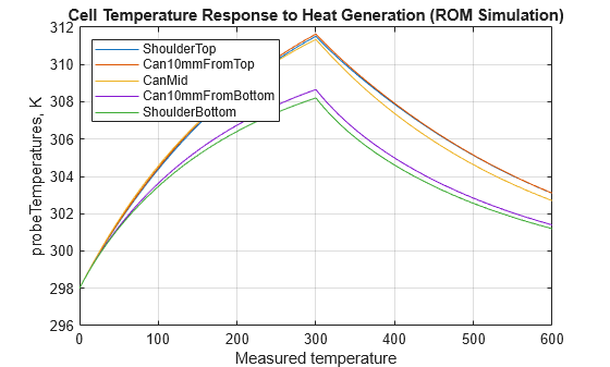
Simulate the model and plot the temperature evolution. The temperature increases at the beginning of the simulation during discharge, and subsequently decreases when the battery is at rest.
cellModelSimOut = sim(cellModelName);
cellModelSimOut.simlog.Thermal_ROM.probeTemperatures.plot;
title("Cell Temperature Response to Heat Generation (ROM Simulation)")
xlabel("Measured temperature")
legend(["ShoulderTop","Can10mmFromTop","CanMid","Can10mmFromBottom","ShoulderBottom"],"Location","northwest")
grid on