Open the model used in the Change Flow Direction tutorial, by typing ssc_gas_tutorial_step3.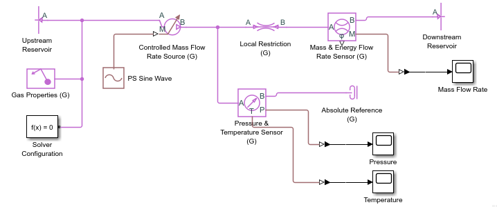

First, to remove the clutter from the block diagram, delete the sensor blocks and scopes. Simulation data logging lets you view and analyze the simulation results without using sensor and scopes.

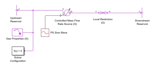
Turn on simulation data logging. Select the Local Restriction (G) block and, on the Simscape Block tab of the model toolstrip, open the Log Data menu. Select Log Data and Log all Simscape data.

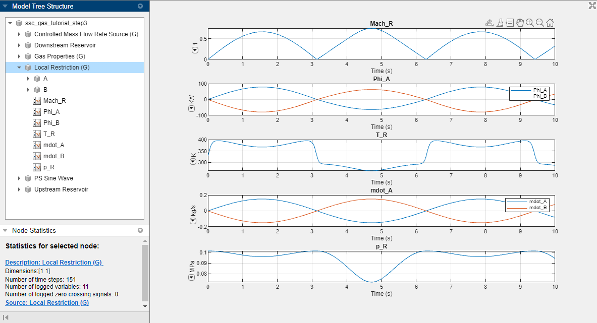
Simulate the model. Then, on the Simscape Block tab, click Results Explorer.

The Simscape™ Results Explorer window opens. It allows you to see many more variables describing the behavior of the blocks without having to connect sensors.

Now, to turn the model into a closed system, delete the reservoir blocks and reconnect the Local Restriction (G) block back to the Controlled Mass Flow Rate Source (G) block.

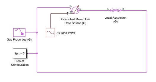
Simulate the model again. Unlike in the previous step, you now get an error solving the system, as well as warnings about dependent or inconsistent equations. This issue arose because with the removal of the reservoir blocks, the model no longer has a reference node. There must be at least one block in the model with gas volume. The gas volume serves as a reference node.

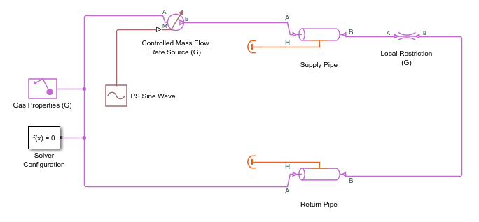
To resolve the issue, add a Pipe (G) block before and after the restriction. The Pipe (G) block models a finite gas volume, so it serves as a reference node. One block would have been sufficient, but it is more realistic to have one pipe before and one after the restriction. Rename the blocks to Supply Pipe and Return Pipe, respectively. Assume the pipes are perfectly insulated by connecting Perfect Insulator blocks to their thermal port.

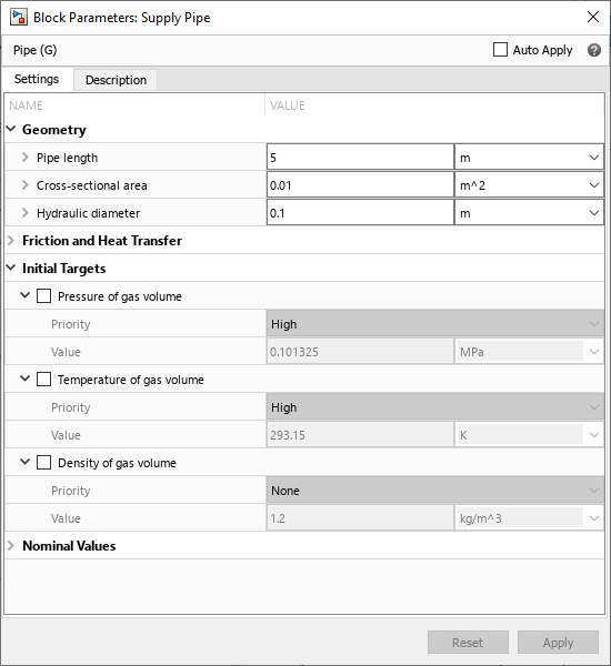
Because the Pipe (G) block has a finite gas volume, it needs initial conditions, which you can specify in the Initial Targets section of the block dialog box. By default, the block sets high-priority initial targets for pressure and temperature. Double-click the Supply Pipe block and expand the Initial Targets section to view the initialization targets.

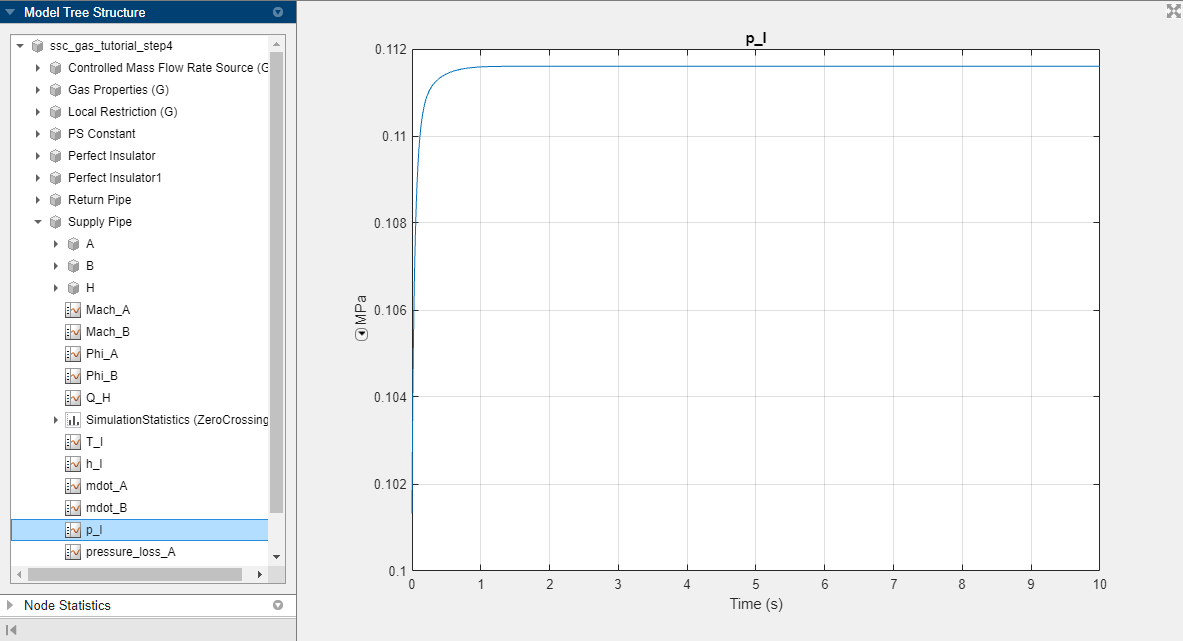
Simulate the model and view the simulation results.

The subscript I indicates the internal node of the block, which represents the state of the gas volume. Therefore, T_I is the gas volume temperature and rho_I is the gas density inside the pipe.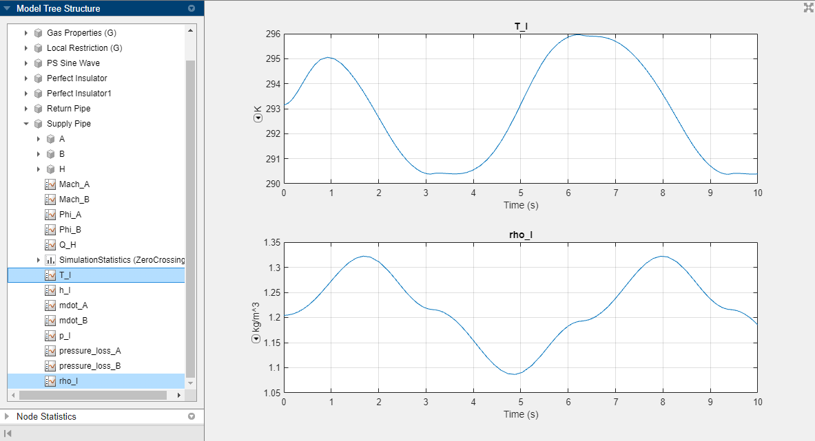

To explore the effect of initialization targets on the simulation results, you can change the target values or change which of the initial conditions have high priority.

For example, change temperature priority to None and change density to have High priority and a value of 1.3 kg/m^3.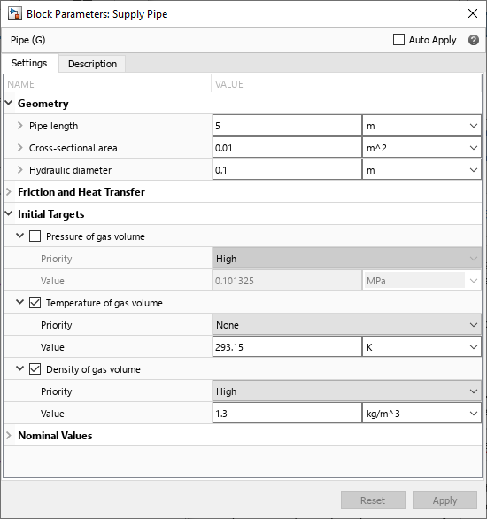

Simulate the model again.

The gas volume density rho_I now starts at 1.3 kg/m^3. The temperature T_I no longer starts at 293.15 K. It now starts at 271.6 K, to be consistent with the specified pressure and density.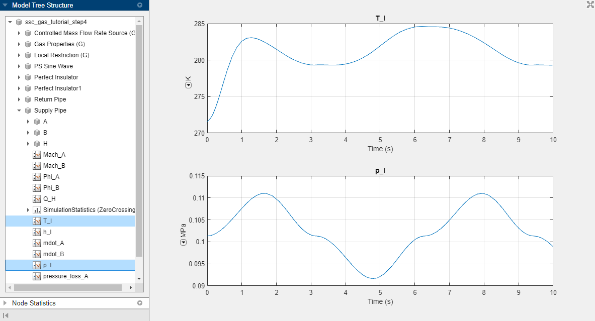

You can specify high-priority targets only for two out of the three variables. If you set priority to High for all three variables, the system becomes over-specified. For more information, see Initialize Variables for a Mass-Spring-Damper System. Conversely, if you specify less than two high-priority variables, the initial conditions are under-constrained and the solver might initialize to values that you do not expect.

Clear the check boxes to revert to the default initial conditions.

Change the input to the Controlled Mass Flow Rate Source (G) block from a sine wave to a constant signal, by replacing the PS Sine Wave block with a PS Constant block. Set the Constant parameter to 0.15 kg/s.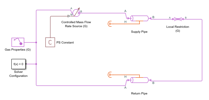

Simulate the model and view the simulation results.

Mass flow rate through port A of the Supply Pipe block, mdot_A, has a constant value of 0.15 kg/s because the mass flow rate source is connected to this port.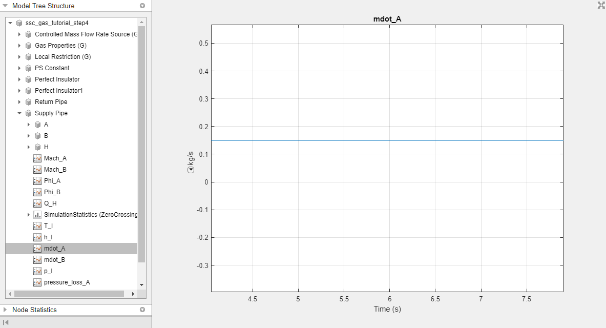

However, mass flow rate through port B, mdot_B, starts at 0 kg/s and quickly decreases to -0.15 kg/s. The flow rate is negative because of the sign convention: positive in and negative out.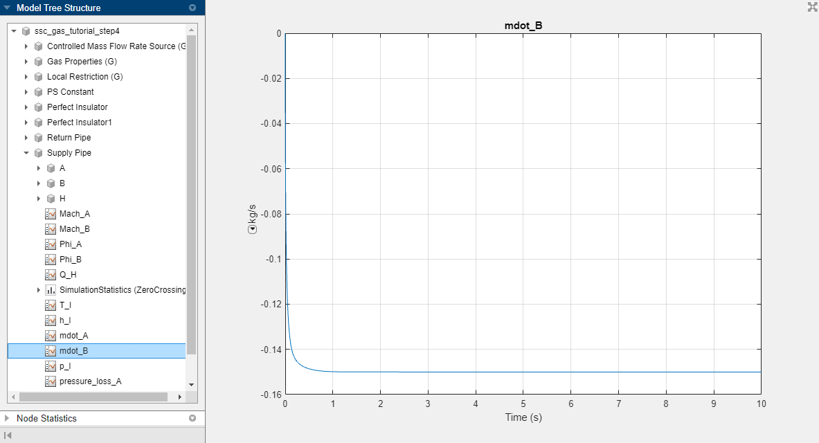

The reason mdot_B does not start at -0.15 kg/s is because the block models the compressibility of the gas volume inside the pipe. As the source pushes mass flow into port A, it takes time for the pressure to build up and cause mass flow out of port B. Look at p_I to see this build up in pressure of the gas volume inside the pipe.