Linearize an Electronic Circuit
This example shows how to linearize a model of a nonlinear bipolar transistor circuit and create a Bode plot for small-signal frequency-domain analysis.
Depending on the software you have available, use the appropriate sections of this example to explore various linearization and analysis techniques.
Explore the Model
To open the Nonlinear Bipolar Transistor example model, type:
openExample('simscape/NonlinearBipolarTransistorExample')
The model represents a single-transistor audio amplifier. The transistor is an NPN bipolar device, and as such has a nonlinear set of current-voltage characteristics. Therefore the overall behavior of the amplifier is dependent on the operating point of the transistor. The transistor itself is represented by and Ebers-Moll equivalent circuit implemented using a masked subsystem. The circuit has a sinusoidal input test signal with amplitude 10 mV and frequency 1 kHz. The Load Voltage scope displays the resulting collector output voltage after the DC is filtered out by the output decoupling capacitor.
R1 and R2 set the nominal operating point, and the small signal gain is approximately set by the ratio R3/R4. The decoupling capacitors C1 and C2 have a capacitance of 1uF, to present negligible impedance at 1 kHz.
The model is configured for linearization. You can quickly generate and view the
small-signal frequency response by clicking the Linearize circuit
hyperlink in model annotation. To view the MATLAB® script that generates the frequency response, click the next hyperlink
in that annotation, see code. This documentation provides
background information and alternative ways of linearization based on the software
you have.
In general, to obtain a nontrivial linearized input-output model and generate a frequency response, you must specify model-level inputs and outputs. The Nonlinear Bipolar Transistor model meets this requirement in two ways, depending on how you linearize:
Simulink® requires top- or model-level input and output ports for linearization with
linmod. The Nonlinear Bipolar Transistor model has such ports, markeduandy.Simulink Control Design™ software requires that you specify input and output signal lines with linearization points. The specified lines must be Simulink signal lines, not Simscape™ physical connection lines. The Nonlinear Bipolar Transistor model has such linearization points specified. For more information on using Simulink Control Design software for trimming and linearization, see documentation for that product.
Open the Solver Configuration block and see that the Start simulation from steady state check box is selected. Then open the Load Voltage scope and run the simulation to see the basic circuit behavior. The transistor junction capacitance initial voltages are set to be consistent with the bias conditions defined by the resistors. The output is a steady sinusoid with zero average, its amplitude amplified by the transistor and bias circuit.

To see the circuit relax from a nonsteady initial state, in the Solver Configuration block, clear the Start simulation from steady state check box and click Apply. With the Load Voltage scope open, simulate again. In this case, the output voltage starts at zero because the transistor junction capacitances start with zero charge.
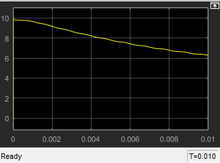
You can get a more comprehensive understanding of the circuit behavior and how it approaches the steady state by long-time transient simulation. Increase the simulation time to 1 s and rerun the simulation. The circuit starts from its initial nonsteady state, and the transistor collector voltage approaches and eventually settles into steady sinusoidal oscillation.

Open the Solver Configuration block, select the Start simulation from steady state check box (as it was when you first opened the model), and click Apply. Change the simulation time back to .01 s and rerun the simulation.
Linearize with Steady-State Solver and linmod Function
In this example, you:
Use the Simscape steady-state solver to find an operating point
Linearize the model using the Simulink
linmodfunctionGenerate the Bode plot using a series of MATLAB commands
Open the Solver Configuration block and make sure the Start simulation from steady state check box is selected. When you simulate the model with the Simscape steady-state solver enabled, the circuit is initialized at the state defined by the transistor bias resistors. This steady-state solution is an operating point suitable for linearization.
Note
Also make sure that the Use local solver check box is cleared. Linearizing a model with the local solver enabled is not supported.
To linearize the model, type:
[a,b,c,d]=linmod('NonlinearBipolarTransistor');You can alternatively call the linmod function with a single
output argument, in which case it generates a structure with states, inputs, and
outputs, as well as the linear time-invariant (LTI) model.
The state vector of the Nonlinear Bipolar Transistor model contains 11 components. The full model has one input and one output. Thus, the LTI state-space model derived from linearization has the following matrix sizes:
a is 11-by-11
b is 11-by-1
c is 1-by-11
d is 1-by-1
To generate a Bode plot, type the following in the MATLAB Command Window:
npts = 100; f = logspace(-2,10,npts); G = zeros(1,npts);
for i=1:npts
    G(i) = c*(2*pi*1i*f(i)*eye(size(a))-a)^-1*b +d;
end
subplot(211), semilogx(f,20*log10(abs(G)))
grid
ylabel('Magnitude (dB)')
subplot(212), semilogx(f,180/pi*unwrap(angle(G)))
ylabel('Phase (degrees)')
xlabel('Frequency (Hz)')
grid 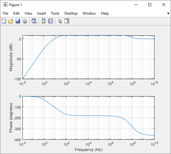
Note
The linmod function provides only basic linearization
capabilities. For full linearization functionality, use Simulink
Control Design software. For more information, see Choose Linearization Tools (Simulink Control Design).
Linearize with Simulink Control Design Software
Note
To work through this section, you must have a Simulink Control Design license.
Simulink Control Design software has tools that help you find operating points and returns a state-space model object that defines state names. This is the recommended way to linearize Simscape models.
In the Simulink Toolstrip of the Nonlinear Bipolar Transistor model window, on the Apps tab, under Control Systems, click Model Linearizer.
In the Model Linearizer window, on the Linear Analysis tab, click the Bode plot button.
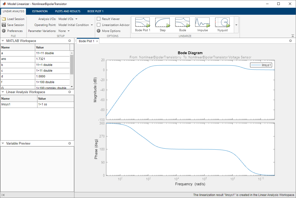
For more information on using Simulink Control Design software for trimming and linearization, see the Simulink Control Design documentation.
Use Control System Toolbox Software for Bode Analysis
Note
To work through this section, you must have a Control System Toolbox™ license.
You can use the built-in analysis and plotting capabilities of Control System Toolbox software to analyze and compare Bode plots of different steady states.
First, use the Simulink
linmod function to obtain the linear time-invariant (LTI)
model.
[a,b,c,d]=linmod('NonlinearBipolarTransistor');Not all the states of the LTI model derived in this example are independent.
Confirm this by calculating the determinant of the a matrix,
det(a). The determinant vanishes, which implies one or more
zero eigenvalues. To analyze the LTI model, reduce the LTI matrices to a minimal
realization. Obtain a minimal realization using the minreal
function.
[a0,b0,c0,d0] = minreal(a,b,c,d);
7 states removed.
Extracting the minimal realization eliminates 7 dependent states from the LTI
model, leaving four independent states. Analyze the control characteristics of the
reduced a0, b0, c0,
d0 LTI model using a Bode plot.
bode(a0,b0,c0,d0) % Creates first Bode plotThe circuit with R1 changed from 47 to 15 kOhm has a different steady state and response. Double-click the R1 block, change the Resistance value to 15 kOhm, and click Apply. Open the Load Voltage scope and simulate the model. The collector voltage is now no longer amplified relative to the 10 mV AC source but attenuated.
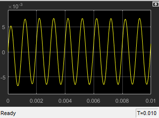
Produce the LTI model at the second steady state, reduce it to a minimal realization, and superpose the second Bode plot on the first one.
[a_R1,b_R1,c_R1,d_R1]=linmod('NonlinearBipolarTransistor');
[a0_R1,b0_R1,c0_R1,d0_R1] = minreal(a_R1,b_R1,c_R1,d_R1); % 7 states removed.
hold on % Keeps first Bode plot open
bode(a0_R1,b0_R1,c0_R1,d0_R1) % Superposes second Bode plot on first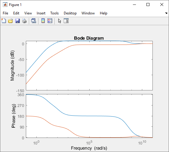
For more information on using Control System Toolbox software for Bode analysis, see the Control System Toolbox documentation.