Projection

R2026b

Perturb the solver's solution of a system's states to better satisfy time-invariant solution relationships

Required

Language

MATLAB^®

Syntax

Projection(s)

Arguments

s: Instance of Simulink.MSFcnRunTimeBlock class representing the Level-2 MATLAB S-Function block.

Description

This method is intended for use with S-functions that model dynamic systems whose states satisfy time-invariant relationships, such as those resulting from mass or energy conservation or other physical laws. The Simulink^® engine invokes this method at each time step after the model's solver has computed the S-function's states for that time step. Typically, slight errors in the numerical solution of the states cause the solutions to fail to satisfy solution invariants exactly. Your Projection method can compensate for the errors by perturbing the states so that they more closely approximate solution invariants at the current time step. As a result, the numerical solution adheres more closely to the ideal solution as the simulation progresses, producing a more accurate overall simulation of the system modeled by your S-function.

Your Projection method's perturbations of system states must fall within the solution error tolerances specified by the model in which the S-function is embedded. Otherwise, the perturbations may invalidate the solver's solution. It is up to your Projection method to ensure that the perturbations meet the error tolerances specified by the model. See Perturbing a System's States Using a Solution Invariant for a simple method for perturbing a system's states. The following articles describe more sophisticated perturbation methods that your mdlProjection method can use.

C.W. Gear. “Maintaining Solution Invariants in the Numerical Solution of ODEs.” Journal on Scientific and Statistical Computing 7, no. 3 (July 1986).
L.F. Shampine. “Conservation Laws and the Numerical Solution of ODEs I.” Computers and Mathematics with Applications 12B (1986): 1287–96.
L.F. Shampine. “Conservation Laws and the Numerical Solution of ODEs II.” Computers and Mathematics with Applications 38 (1999) 61–72.

Examples

collapse all

Perturbing a System's States Using a Solution Invariant

Here is a simple, Taylor-series-based approach to perturbing a system's states. Suppose your S-function models a dynamic system having a solution invariant, $g (X, t)$ , i.e., $g$ is a continuous, differentiable function of the system states, $X$ , and time, $t$ , whose value is constant with time. Then

$X_{n} ≅ X_{n}^{*} + J_{n}^{T} {(J_{n} J_{n}^{T})}^{- 1} R_{n}$

where

$X_{n}$ is the system's ideal state vector at the solver's current time step
$X_{n}^{*}$ is the approximate state vector computed by the solver at the current time step
$J_{n}$ is the Jacobian of the invariant function evaluated at the point in state space specified by the approximate state vector at the current time step:
$J_{n} = \frac{\partial g}{\partial X} (X_{n}^{*}, t_{n})$
$t_{n}$ is the time at the current time step
$R_{n}$ is the residual (difference) between the invariant function evaluated at $X_{n}$ and $X_{n}^{*}$ at the current time step:
$R_{n} = g (X_{n}, t_{n}) - g (X_{n}^{*}, t_{n})$
Note
The value of $g (X_{n}, t_{n})$ is the same at each time step and is known by definition.

Given a continuous, differentiable invariant function for the system that your S-function models, this formula allows your S-function's mdlProjection method to compute a perturbation

$J_{n}^{T} {(J_{n} J_{n}^{T})}^{- 1} R_{n}$

of the solver's numerical solution, $X_{n}^{*}$ , that more closely matches the ideal solution, $X_{n}$ , keeping the S-function's solution from drifting from the ideal solution as the simulation progresses.

Setup Working Environment for Perturbation Method Example

Open Live Script

This example opens up a directory containing the following files required for this example.

mdlProjectionEx1.slx
mdlProjectionEx2.slx
predprey_noproj.m
predprey.m

Setup Working Environment for Perturbation Method Example

Open Live Script

This example opens up a directory containing the following files required for this example.

mdlProjectionEx1.slx
mdlProjectionEx2.slx
predprey_noproj.m
predprey.m

Perturbation Method Example

This example illustrates how the perturbation method outlined in the previous section can keep a model's numerical solution from drifting from the ideal solution as a simulation progresses. Consider the following model, mdlProjectionEx1:

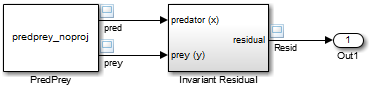
The PredPrey block references an S-function that uses the Lotka-Volterra equations:

predprey_noproj.m

function predprey_noproj(block)
% This is one of a pair S-functions that model a population of predators
% and preys, the other being predprey.m.

% Both S-functions use the Lotka-Volterra equations
%
%   xdot = ax(1-y)
%   ydot = -cy(1-x)
%
% to model changes in the population where x(t) and y(t) are 
% the number of predators and prey, respectively, and 
% a and c are constants. Both S-functions assume a=1 and c=2 and
% that the population consists initially of one predator and three prey.
% 
% The solution to the Lotka-Volterra equations obeys the time-invariant
% relationship
%
%   (x^-c)*exp(cx)*(y^-a)*exp(ay) = d
%
% where d is a constant.
%
% The other S-function uses this relationship to compensate for
% numerical errors in the solver's solution of the model's state
% equations. This S-function does not attempt to compensate for the
% numerical errors. As a result, the solution drifts from the ideal
% solution as the simulation progresses.
%
% For more information, see the documentation for the mdlProjection 
% method in the online Simulink documentation.
%   
% Copyright 2006 The MathWorks, Inc.

  setup(block);
  
%endfunction

function setup(block)
  
  %% Register number of input and output ports
  block.NumInputPorts  = 0;
  block.NumOutputPorts = 2;

  block.OutputPort(1).Dimensions       = 1;
  block.OutputPort(1).SamplingMode = 'Sample';
  
  block.OutputPort(2).Dimensions       = 1;
  block.OutputPort(2).SamplingMode = 'Sample';

  
  %% Set block sample time to variable sample time
  block.SampleTimes = [0 0];
  
  %% Setup Dwork
  block.NumContStates = 2;
  
  %% Register methods
  block.RegBlockMethod('InitializeConditions',    @InitConditions); 
  block.RegBlockMethod('Outputs',                 @Output);  
  block.RegBlockMethod('Derivatives', @Derivatives);
  block.RegBlockMethod('Projection', @Projection);
  block.RegBlockMethod('Update', @Update);
  
%endfunction

function InitConditions(block)

  %% Initialize Dwork: 1 predator, 3 prey.
  block.ContStates.Data = [1 3]';
  
  
%endfunction

function Output(block)

  % Output number of predators.
  block.OutputPort(1).Data = block.ContStates.Data(1);
  
  % Output number of prey.
  block.OutputPort(2).Data = block.ContStates.Data(2);
  
  block.ContStates.Data;
  
%endfunction

function Derivatives(block)

states = block.ContStates.Data;
% System ODEs
block.Derivatives.Data = [2*states(1)*(1-states(2)); -states(2)*(1-states(1))];
  
%endfunction

function Projection(block)
    %not implemented
%endfunction

function Update(block)

%endfunction

$\begin{array}{l} \dot{x} = a x (1 - y) \\ \dot{y} = - c y (1 - x) \end{array}$

to model predator-prey population dynamics, where $x (t)$ is the population density of the predators and $y (t)$ is the population density of prey. The ideal solution to the predator-prey ODEs satisfies the time-invariant function

$x^{- c} e^{c x} y^{- a} e^{a y} = d$

where $a$ , $c$ , and $d$ are constants. The S-function assumes a = 1, c = 2, and d = 121.85.

The Invariant Residual block in this model computes the residual between the invariant function evaluated along the system's ideal trajectory through state space and its simulated trajectory:

$R_{n} = d - x_{n}^{- c} e^{c x_{n}} y_{n}^{- a} e^{a y_{n}}$

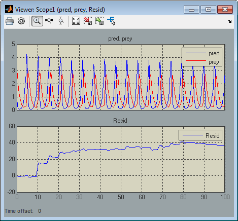
where $x_{n}$ and $y_{n}$ are the values computed by the model's solver for the predator and prey population densities, respectively, at the current time step. Ideally, the residual should be zero throughout simulation of the model, but simulating the model reveals that the residual actually strays considerably from zero:

Now consider the following model, mdlProjectionEx2:

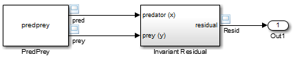
This model is the same as the previous model, except that its S-function, predprey.m, includes a mdlProjection method that uses the perturbation approach outlined in Perturbing a System's States Using a Solution Invariant to compensate for numerical drift. As a result, the numerical solution more closely tracks the ideal solution as the simulation progresses as demonstrated by the residual signal, which remains near or at zero throughout the simulation:

predprey.m

function predprey(block)
% This is one of a pair S-functions that model a population of predators
% and preys, the other being predprey_noproj.m.

% Both S-functions use the Lotka-Volterra equations
%
%   xdot = ax(1-y)
%   ydot = -cy(1-x)
%
% to model changes in the population where x(t) and y(t) are 
% the number of predators and prey, respectively, and 
% a and c are constants. Both S-functions assume a=1 and c=2 and
% that the population consists initially of one predator and three prey.
% 
% The solution to the Lotka-Volterra equations obeys the time-invariant
% relationship
%
%   (x^-c)*exp(cx)*(y^-a)*exp(ay) = d
%
% where d is a constant.
%
% This S-function uses this relationship to compensate for
% numerical errors in the solver's solution of the model's state
% equations. The other S-function does not. As a result, 
% the other's solution drifts from the ideal solution as the 
% simulation progresses.
%
% For more information, see the documentation for the mdlProjection 
% method in the online Simulink documentation.
%   
% Copyright 2006 The MathWorks, Inc.
  setup(block);
  
%endfunction

function setup(block)
  
  %% Register number of input and output ports
  block.NumInputPorts  = 0;
  block.NumOutputPorts = 2;

  block.OutputPort(1).Dimensions       = 1;
  block.OutputPort(1).SamplingMode = 'Sample';
  
  block.OutputPort(2).Dimensions       = 1;
  block.OutputPort(2).SamplingMode = 'Sample';

  
  %% Set block sample time to variable sample time
  block.SampleTimes = [0 0];
  
  %% Setup Dwork
  block.NumContStates = 2;
  
  %% Register methods
  block.RegBlockMethod('InitializeConditions',    @InitConditions); 
  block.RegBlockMethod('Outputs',                 @Output);  
  block.RegBlockMethod('Derivatives', @Derivatives);
  block.RegBlockMethod('Projection', @Projection);
  
%endfunction

function InitConditions(block)

  %% Initialize Dwork: 1 predator, 3 prey.
  block.ContStates.Data = [1 3]';
  
  
%endfunction

function Output(block)

  % Output number of predators.
  block.OutputPort(1).Data = block.ContStates.Data(1);
  
  % Output number of prey.
  block.OutputPort(2).Data = block.ContStates.Data(2);
  block.ContStates.Data;
  
%endfunction

function Derivatives(block)

states = block.ContStates.Data;
% System ODEs
block.Derivatives.Data = [2*states(1)*(1-states(2)); -states(2)*(1-states(1))];
  
%endfunction

function Projection(block)

states = block.ContStates.Data;

%Computing the Jacobian of the Invariant
J = localInvJac(states);

%Computing the residual of the invariant
R = localInvRes(states);

%Perturbing the states
states = states + (J')*((J*(J'))^-1) * R;

%Update the states
block.ContStates.Data = states; 

%endfunction

function J = localInvJac(states)

%Computing the Jacobian of the invariant
L = 1/states(1) * exp(states(1));
R = 1/(states(2)^2)*exp(2*states(2));
Lx = (states(1)-1)/(states(1)^2)*exp(states(1));
Ry = 2*(states(2)-1)/(states(2)^3)*exp(2*states(2));

J = [Lx*R L*Ry];

%endfunction

function R = localInvRes(states)

%Invariant value
inv0 = 1.218481287142732e+002;

%Computing invariant
L = 1/states(1) * exp(states(1));
R = 1/(states(2)^2)*exp(2*states(2));
inv = L*R;

%Residual
R = inv0-inv;

%endfunction

Version History

Introduced in R2012b

Projection

Required

Language

Syntax

Arguments

Description

Examples

Perturbing a System's States Using a Solution Invariant

Setup Working Environment for Perturbation Method Example

Setup Working Environment for Perturbation Method Example

Perturbation Method Example

See Also

Version History