Algebraic Constraint
R2026bConstrain signal value when solving algebraic loop
Algebraic Constraint block

To add a block to a model, double-click the canvas and start typing the block name. Then, select the block from the list.
Libraries:
Simulink /
Math Operations
Description
The Algebraic Constraint block constrains the value of the input when solving an algebraic loop that contains the block. You can configure the block to apply either of these constraint equations:
f(z) = 0,
f(z) = z,
where:
z is an algebraic variable or vector of algebraic variables in the loop.
f(z) is the block input signal.
The block determines the value of the algebraic variable z that satisfies the specified constraint equation and provides the value as an output.
Solve Algebraic Loops as Differential-Algebraic Equations (DAEs)
Solving an algebraic loop as a DAE can significantly speed up simulations in some cases for models that:
Have continuous states
Use Algebraic Constraint blocks to constrain the value of coupled states between State-Space or Descriptor State-Space blocks
By default, the software solves algebraic loops as a system of equations expressed in the semi-explicit form:
To solve the algebraic equations, the software invokes the algebraic loop solver.
To solve an algebraic loop as a DAE instead, set the Equation
format parameter of each Algebraic Constraint block in
the loop to Differential Algebraic Equation. The software
solves the loop as a system of DAEs in the form:
where the algebraic variable z is treated as one of the continuous system states x.
To solve the loop, the software uses the solver specified to simulate the model. To solve algebraic loops as DAEs, you must simulate the model using an implicit solver.
Examples
Use the Algebraic Constraint block to solve the system

The model represents the problem in a vectorized form as
![$$ \left[\begin{array}{cc} 1 & 1\\ -1& 1 \end{array}\right]\left[\begin{array}{c}z_1\\z_2\end{array}\right] =\left[\begin{array}{c}1\\1\end{array}\right] $$](../../examples/simulink/SolveALinearSystemOfAlgebraicEquationsExample_eq00627851823494940069.png)
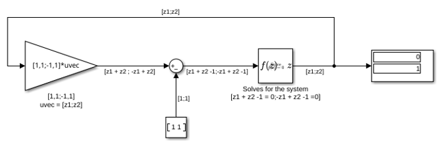
The signal fed to the Algebraic Constraint block  is a
is a  vector of the form
![$$\left[\begin{array}{c}z_1+z_2-1\\-z-1 + z_2-1\end{array}\right] $$](../../examples/simulink/SolveALinearSystemOfAlgebraicEquationsExample_eq14029990663688292877.png)
The block is configured to constrain to 0. Thus solving for  yields the solution
Extended Examples
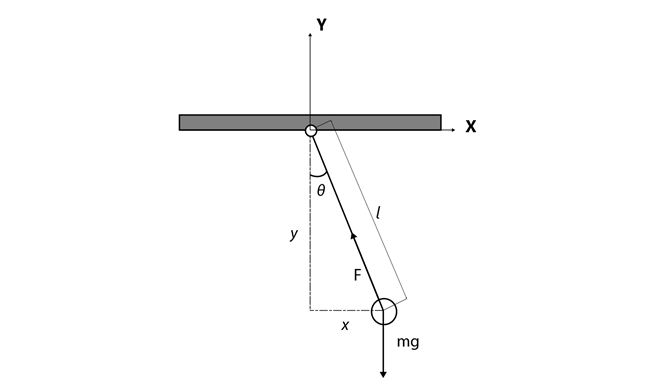
Model a Planar Pendulum
Consider a point mass m suspended by a massless rod of length l under the influence of gravity.
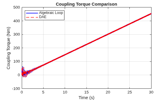
Solve Algebraic Loops as Differential-Algebraic Equations (DAEs)
Solve the algebraic loop in a practical drivetrain model as a differential-algebraic equation (DAE). The example compares the DAE approach to the algebraic loop solver and explains how to decide when to use each option.
Ports
Input
Output
Parameters
Block Characteristics
Data Types |
|
Direct Feedthrough |
|
Multidimensional Signals |
|
Variable-Size Signals |
|
Zero-Crossing Detection |
|
References
[1] Garbow, B. S., K. E. Hillstrom, and J. J. Moré. User Guide for MINPACK-1. Argonne, IL: Argonne National Laboratory, 1980.
[2] Rabinowitz, P. H. Numerical Methods for Nonlinear Algebraic Equations. New York: Gordon and Breach, 1970.
[3] Kelley, C. T. Iterative Methods for Linear and Nonlinear Equations. Society for Industrial and Applied Mathematics, Philadelphia, PA: 1995.

