Implement Fixed-Step Implicit Trapezoidal Solver

R2026b

This example shows how to write a plugin solver with a fixed-step integration algorithm that implements the trapezoidal rule and use the solver to simulate a model of a harmonic oscillator. Built-in solvers can simulate a wide range of systems, but are not necessarily ideal for all domains and problems. The trapezoidal rule is well suited to oscillatory systems because it preserves energy and does not introduce artificial damping in the oscillations.

Harmonic Oscillator and Trapezoidal Rule

These equations govern the dynamics of the undamped harmonic oscillator:

$x_{}^{¨} + ω^{2} x = 0$

$x (0) = 1$

$x_{}^{˙} (0) = 0,$

where $x$ is the displacement and $ω$ is the angular frequency.

Open the model HarmonicOscillator. The model implements an undamped harmonic oscillator with a period of 1 second. For this model, the exact solution is $x (t) = \cos (2 π t)$ .

mdl = "HarmonicOscillator";
open_system(mdl)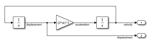

Block diagram of the model HarmonicOscillator.

The trapezoidal rule numerically integrates by approximating a region under a curve as a trapezoid and calculating its area according to this equation:

$x_{n + 1} = x_{n} + \frac{h}{2} (f_{n} + f_{n + 1}),$

where:

$x_{n}$ is the state vector at time $t_{n}$ .
$x_{n + 1}$ is the state vector at time $t_{n + 1}$ .
$h$ is the fixed step size.
$f_{n}$ is the forcing function evaluated at time $t_{n}$ with state $x_{n}$ .
$f_{n + 1}$ is the forcing function evaluated at time $t_{n + 1}$ with state $x_{n + 1}$ .

Because $f_{n + 1}$ depends on $x_{n + 1}$ , a trapezoidal rule solver must solve for $x_{n + 1}$ using Newton iterations and the system Jacobian in each time step.

`PluginODE2T` Solver Class

The plugin solver PluginODE2T inherits from the Simulink.Solver.FixedStepSolver base class. The trapezoidal rule is an implicit technique that requires Newton iterations. The PluginODE2T class defines a property named MaxNewtonIterations that specifies the maximum number of iterations per step.

properties (Access = private)
    MaxNewtonIterations = 20
end

The integration algorithm evaluates the system Jacobian and mass matrix. To enable access to the massMatrix and Jacobian methods, the solver defines these properties in the getProperties method.

function props = getProperties()
    props = struct("MassMatrix",true,"Jacobian",true);
end

The step method implements the implicit integration algorithm based on the trapezoidal rule. At the start of each step, the algorithm:

Advances time using the fixed step size
Computes the state derivative ${x_{}^{˙}}_{0} = M_{0} \ f_{0}$ by calling the massMatrix and forcingFunction methods
Computes an initial guess for $x_{n + 1}$ using the state derivative

Starting with the initial guess, each Newton iteration solves the root equation:

$G (x_{n + 1}) = M_{n + 1} (x_{n + 1} - x_{n} - \frac{h}{2} {x_{}^{˙}}_{n}) - \frac{h}{2} f_{n + 1} = 0,$

where $G (x_{n + 1})$ is the system equation $x_{}^{¨} + ω^{2} x = 0$ . In each iteration, the solver refines the current estimate of $x_{n + 1}$ using the iteration matrix:

$M_{n + 1} - \frac{h}{2} J_{n + 1} .$

function xout = step(slvr,t0,x0,stepSize)
    n = slvr.NumStates;
    h = stepSize;
    t1 = t0 + h;

    f0 = forcingFunction(slvr,t0,x0);
    M0 = reshape(massMatrix(slvr,t0,x0),n,n);
    xdot0 = M0 \ f0;

    xnew = x0 + h * xdot0;

    for iter = 1:slvr.MaxNewtonIterations
        f1 = forcingFunction(slvr,t1,xnew);
        M1 = reshape(massMatrix(slvr,t1,xnew),n,n);
        J1 = reshape(Jacobian(slvr,t1,xnew),n,n);

        residual = M1 * (xnew - x0 - (h/2) * xdot0) - (h/2) * f1;

        iterationMatrix = M1 - (h/2) * J1;
        delta = iterationMatrix \ residual;
                
        xnew = xnew - delta;

        if all(abs(delta) <= 16 * eps(abs(xnew)))
            break
        end
    end
    xout = xnew;
end

Simulate Harmonic Oscillator Model

To analyze how the PluginODE2T solver compares to the built-in ode1be and ode14x solvers, simulate the harmonic oscillator model using each solver.

To use a plugin solver, register the solver. After you register a plugin solver, you can specify the solver using set_param or select the solver from the Solver list in the Configuration Parameters dialog box.

Register the plugin solver PluginODE2T. To select the plugin solver, specify the SolverType and SolverName parameters.

Simulink.Solver.register("PluginODE2T")
set_param(mdl,SolverType="Fixed-step")
set_param(mdl,SolverName="PluginODE2T")

Configure the model to simulate with a fixed step size of 0.01 seconds, which results in 100 time steps per oscillation period. Then, simulate the model using the plugin solver.

set_param(mdl,FixedStep="0.01")
outTrap = sim(mdl);

Simulate the model using the built-in ode1be solver.

set_param(mdl, Solver="ode1be")
outBE = sim(mdl);

Simulate the model using the built-in ode14x solver.

set_param(mdl, Solver="ode14x")
out14x = sim(mdl);

Analyze Simulation Results

To analyze how each solver performed in each simulation, compare the results from each simulation against the exact solution.

Compute the exact solution between 0 and 10 seconds.

tExact = linspace(0,10,2000);
xExact = cos(2*pi*tExact);

Get the logged velocity and displacement for each simulation.

vTrap = outTrap.yout{1}.Values.Data;
xTrap = outTrap.yout{2}.Values.Data;
vBE = outBE.yout{1}.Values.Data;
xBE = outBE.yout{2}.Values.Data;
v14x = out14x.yout{1}.Values.Data;
x14x = out14x.yout{2}.Values.Data;

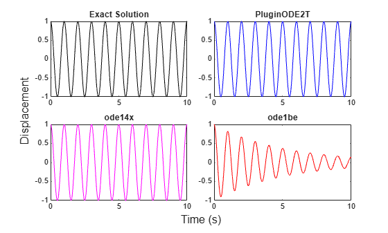
Plot the exact solution and the results from each simulation. Over the 10-second simulation, the plugin solver and ode14x solver preserve the constant amplitude of the exact solution. The ode1be solver introduces significant decay in the amplitude.

p = tiledlayout(TileSpacing="compact")

p = 
  TiledChartLayout with properties:

    TileArrangement: 'flow'
           GridSize: [1 1]
            Padding: 'loose'
        TileSpacing: 'compact'

  Show all properties

nexttile
plot(tExact,xExact,"k-")
title("Exact Solution")
nexttile
plot(outTrap.tout,xTrap,"b-")
title("PluginODE2T")
nexttile
plot(out14x.tout,x14x,"m-")
title("ode14x")
nexttile
plot(outBE.tout,xBE,"r-")
title("ode1be")
xlabel(p,"Time (s)")
ylabel(p,"Displacement")

Figure contains 4 axes objects. Axes object 1 with title Exact Solution contains an object of type line. Axes object 2 with title PluginODE2T contains an object of type line. Axes object 3 with title ode14x contains an object of type line. Axes object 4 with title ode1be contains an object of type line.

Analyze Energy Preservation

The total energy of the harmonic oscillator is given by the equation:

$E = \frac{1}{2} ({x_{}^{˙}}^{2} + ω^{2} x^{2}) .$

For the exact solution, $E$ is constant for all time.

Plot the normalized energy $E (t) / E (0)$ for each solver.

omega = 2 * pi;
E0 = 0.5 * omega^2;

eTrap = 0.5 * (vTrap.^2 + omega^2 * xTrap.^2);
eBE = 0.5 * (vBE.^2 + omega^2 * xBE.^2);
e14x = 0.5 * (v14x.^2 + omega^2 * x14x.^2);

figure
plot(outTrap.tout,eTrap/E0,"b-o", ...
    outBE.tout,eBE/E0,"r-", ...
    out14x.tout,e14x/E0,"m-",LineWidth=1.5)
xlabel("Time (s)")
ylabel("Normalized energy E(t) / E(0)")
legend("PluginODE2T","ode1be","ode14x",Location="eastoutside")
ylim([0 1.1])

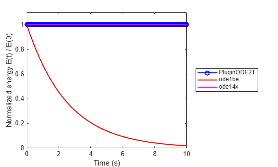
Figure contains an axes object. The axes object with xlabel Time (s), ylabel Normalized energy E(t) / E(0) contains 3 objects of type line. These objects represent PluginODE2T, ode1be, ode14x.

The ode1be solver loses energy monotonically. After only 10 oscillation periods, the solution retains less than 2% of the initial energy.

energyRemainingBE = eBE(end) / eBE(1)

energyRemainingBE = 
0.0194

The ode14x solver shows slow energy growth that causes visible amplitude distortion after thousands of cycles.

drift14x = (e14x(end) - e14x(1)) / e14x(1)

drift14x = 
1.5187e-08

The trapezoidal rule preserves energy to machine precision.

driftTrap = abs(eTrap(end) - eTrap(1)) / eTrap(1)

driftTrap = 
1.4399e-15

Unregister Plugin Solver

To remove a plugin solver from the Solver list, unregister the solver.

Simulink.Solver.unregister("PluginODE2T")

Implement Fixed-Step Implicit Trapezoidal Solver

Harmonic Oscillator and Trapezoidal Rule

`PluginODE2T` Solver Class

Simulate Harmonic Oscillator Model

Analyze Simulation Results

Analyze Energy Preservation

Unregister Plugin Solver

See Also

Classes

Functions

Topics

Implement Fixed-Step Implicit Trapezoidal Solver

Harmonic Oscillator and Trapezoidal Rule

PluginODE2T Solver Class

Simulate Harmonic Oscillator Model

Analyze Simulation Results

Analyze Energy Preservation

Unregister Plugin Solver

See Also

Classes

Functions

Topics

`PluginODE2T` Solver Class