Implement Stabilized Variable-Step Plugin Solver Using Chebyshev Polynomials

Why Standard Explicit Solvers Struggle on Diffusion Problems

Standard explicit Runge-Kutta solvers like ode45 have a narrow stability region along the negative real axis. On diffusion problems whose eigenvalues lie on the negative real axis, the step size is limited by stability, not accuracy. The solver is forced to take many tiny steps even when a larger step would be sufficiently accurate.

The Runge-Kutta-Chebyshev (RKC) scheme extends the stability region along the negative real axis by using Chebyshev polynomial recurrences. With $$s$$ stages, the stability region extends to approximately $$0.65s^2$$ on the negative real axis (the coefficient 0.65 accounts for the damping parameter $$ϵ=2/13$$ used to ensure internal stability of the recurrence). This compares to roughly 3.3 for the Dormand-Prince scheme used by ode45. For the heat equation discretized with $$N=30$$ grid points, using $$s=10$$ stages allows 11x fewer steps than ode45 while remaining fully explicit.

RKC Algorithm

The PluginRKC solver subclasses Simulink.Solver.VariableStepSolver and implements the step method. Key features:

Because the solver is fully explicit, it does not need Jacobian or mass matrix methods. The getProperties method declares this explicitly:

function props = getProperties()
    props = struct("MassMatrix",false,"Jacobian",false);
end

The core of the step method performs adaptive stepping with the built-in error estimate. It returns the time and state of the next time step, where the time is bounded by the time of the prior time step and the maximum step size determined by the simulator.

Each call to rkc2Step evaluates the forcing function $$s$$ times using the Chebyshev recurrence. No matrix operations are needed.

function [tnext, xout] = step(slvr,t0,x0,tnextMax)
    n = slvr.NumStates;
    atol = slvr.AbsoluteTolerance;
    rtol = slvr.RelativeTolerance;
    s = slvr.NumStages;

    hmax = tnextMax - t0;
    if isempty(slvr.PreviousStepSize)
        if isfinite(slvr.InitialStepSize)
            h = min(slvr.InitialStepSize,hmax);
        else
            h = hmax;
        end
    else
        h = min(slvr.PreviousStepSize,hmax);
    end
        h = min(h,slvr.MaxStep);
        h = max(h,slvr.MinStep);

    if isempty(slvr.PreviousF)
        f0 = forcingFunction(slvr,t0,x0);
    else
        f0 = slvr.PreviousF;
    end

    accepted = false;
    while ~accepted
        h = min(h,hmax);
        h = max(h,slvr.MinStep);

        x1 = rkc2Step(slvr,t0,x0,h,s);
        f1 = forcingFunction(slvr,t0 + h,x1);
        err = (1.0/15.0) * (12.0*(x0 - x1) + 6.0*h*(f0 + f1));

        sc = atol + rtol .* max(abs(x0), abs(x1));
        errNorm = norm(err ./ sc) / sqrt(n);

        if errNorm <= 1.0
            accepted = true;
            tnext = t0 + h;
            xout = x1;

            slvr.PreviousF = f1;

            factor = 0.9 * (1.0 / max(errNorm, 1e-10))^(1/3);
            factor = min(factor, 5.0);
            factor = max(factor, 0.2);
            slvr.PreviousStepSize = h * factor;
        else
            factor = 0.9 * (1.0 / errNorm)^(1/3);
            factor = max(factor, 0.2);
            h = h * factor;
        end
    end
end

Register and Simulate

Register the PluginRKC solver and open the heat equation model. The model discretizes the 1-D heat equation $$u_t=\alpha u_{xx}$$ on $$[0,1]$$ with homogeneous Dirichlet boundary conditions using second-order centered finite differences. With $$N=30$$ interior points, the spectral radius is approximately 3844.

Simulink.Solver.register("PluginRKC")
mdl = "HeatEquation1D";
open_system(mdl)

Define the discrete Laplacian matrix used by the Gain block in the model.

N = 30;
alpha = 1.0;
hx = 1.0 / (N + 1);
A = alpha / hx^2 * (diag(ones(N-1,1),1) + diag(ones(N-1,1),-1) - 2*eye(N));

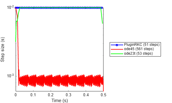
With 10 Chebyshev stages, the RKC solver is stable for step sizes up to $$0.65\times 10^2/\rho \approx 0.017$$ seconds. This is far larger than what ode45 can achieve, so the RKC solver takes uniformly large steps limited only by accuracy.

This highlights the advantage of implementing a custom solver: because you know your problem's spectral radius, you can set the stage count to provide exactly the stability needed. A general-purpose solver cannot exploit this problem-specific knowledge.

set_param(mdl, ...
    StopTime="0.5", ...
    RelTol="1e-3", ...
    AbsTol="1e-3", ...
    MaxStep="auto")
set_param(mdl,Solver="PluginRKC")
outRKC = sim(mdl);

For comparison, simulate with ode45. Its stability region extends only about 3.3 units on the negative real axis, meaning the maximum stable step size is approximately $$3.3/\rho \approx 8.6\times 10^{-4}$$ seconds. The solver is forced to take steps this small to avoid blowing up, regardless of the accuracy tolerance.

set_param(mdl, Solver="ode45")
outODE45 = sim(mdl);

Also simulate with ode23t, an implicit solver based on the trapezoidal rule. Because ode23t is implicit, it is not stability-limited on this problem and can take large steps like RKC.

set_param(mdl,Solver="ode23t")
outODE23t = sim(mdl);

Compare Step-Size Histories

The RKC solver takes uniformly large steps (limited by accuracy), while the step size used by ode45 is limited by stability of the formula. RKC is also cheaper per step than ode23t because it requires no Jacobian evaluation or linear solve. A logarithmic scale reveals the orders-of-magnitude difference in step size.

nStepsRKC = length(outRKC.tout);
nStepsODE45 = length(outODE45.tout);
nStepsODE23t = length(outODE23t.tout);

dtRKC = diff(outRKC.tout);
dtODE45 = diff(outODE45.tout);
dtODE23t = diff(outODE23t.tout);

labelRKC = "PluginRKC (" + nStepsRKC + " steps)";
labelODE45 = "ode45 (" + nStepsODE45 + " steps)";
labelODE23t = "ode23t (" + nStepsODE23t + " steps)";

figure
semilogy(outRKC.tout(1:end-1), dtRKC, "bo-", ...
    outODE45.tout(1:end-1), dtODE45, "r-", ...
    outODE23t.tout(1:end-1), dtODE23t, "g-", ...
    LineWidth=1.5, MarkerSize=4)
xlabel("Time (s)")
ylabel("Step size (s)")
legend(labelRKC, labelODE45, labelODE23t, Location="eastoutside")

Compare Solutions

Verify that all three solvers produce the same solution by plotting the temperature profile at the final time. The analytical solution of the heat equation with initial condition $$u(x,0)=\sin (\pi x)$$ is $$u(x,t)=e^{-{\pi }^{2}t}\sin (\pi x)$$.

xgrid = linspace(0, 1, N+2);
xgrid = xgrid(2:end-1);
uExact = exp(-pi^2*0.5) * sin(pi*xgrid);

yRKC = outRKC.yout{1}.Values.Data(end,:);
yODE45 = outODE45.yout{1}.Values.Data(end,:);
yODE23t = outODE23t.yout{1}.Values.Data(end,:);

figure
plot(xgrid, uExact, "k--", ...
    xgrid, yRKC, "bo", ...
    xgrid, yODE45, "rx", ...
    xgrid, yODE23t, "gs", LineWidth=1.5, MarkerSize=6)
xlabel("Position x")
ylabel("Temperature u(x, t_{final})")
legend("Exact", "PluginRKC", "ode45", "ode23t", Location="eastoutside")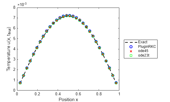

All three solvers converge to the same analytical solution. The small visible differences reflect each solver's tolerance settings. All are within the specified RelTol of $$10^{-3}$$.

Unregister Solver

Unregister the solver to remove it from the Configuration Parameters solver dropdown. This does not delete the solver class file.

Simulink.Solver.unregister("PluginRKC")

References

[1] B.P. Sommeijer, L.F. Shampine, J.G. Verwer. RKC: An Explicit Solver for Parabolic PDEs. Modelling, Analysis and Simulation (MAS), 1997.