Analyze Results Using Model Linearizer Response Plots

Using Model Linearizer, you can analyze time-domain and frequency-domain responses of linearized models. You can compare the responses of multiple models and view system characteristics such as stability margins and settling time.

View System Characteristics on Response Plots

To view system characteristics such as stability margins, overshoot, or settling time on a Model Linearizer response plot, right-click the plot and select Characteristics. Then select the system characteristic you want to view.

For most characteristics, a data marker appears on the plot. To show a data tip that contains information about the system characteristic, click the marker.

Generate Additional Response Plots of Linearized System

In Model Linearizer, when you have linearized or estimated a system, you can generate additional response plots of the system as follows:

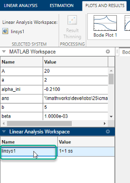
In the Model Linearizer, click the Plots and Results tab. In the Linear Analysis Workspace or the MATLAB Workspace, select the system you want to plot.
In the Plots gallery, click the type of plot you want to generate.
Tip
To expand the gallery view, click .

Model Linearizer generates a new plot of type you select.

Tip

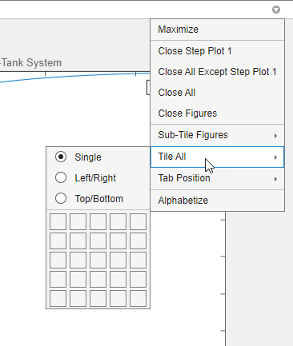
To view multiple plots at the same time, in the top-right corner of the plot document, click the down arrow. Then, select a tiling option under Tile All.

Add Linear System to Existing Response Plot

New Linear System

When you compute a new linearization or frequency response estimation, on the Linear Analysis tab, click the button corresponding to an existing plot to add the new linear system to that plot.

For example, suppose that you have linearized a model at the default operating point for the model, and have a step plot of the result, Step Plot 1. Suppose further that you have specified a new operating point at a linearization snapshot time. To linearize at the new operating point and add the result to Step Plot 1, click Step Plot 1. Model Linearizer computes the new linearization and adds the step response of the new system, linsys2, to the existing step response plot.

Linear System in Workspace

You can add a linear system from the MATLAB Workspace or the Linear Analysis Workspace to an existing plot in Model Linearizer.

On the Plots and Results tab, in the Linear Analysis Workspace, select the system you want to add to an existing plot. Then, in the Plots section of the tab, select the button corresponding to the existing plot you want to update.

For example, suppose that you have a Bode plot of the response of a linear system, Bode Plot 1. Suppose further that you have an estimated response in the Linear Analysis Workspace, estsys1. To add the response of estsys1 to the existing Bode plot, select estsys1 and click Bode Plot 1.

Tip

To expand the gallery view, click .

Customize Characteristics of Plot in Model Linearizer

To change the characteristics of an existing plot, such as the title, axis labels, or text styles, double-click the plot to open the properties editor. Edit plot properties as desired. Plots are updated as you make changes. When you are finished, click Close.

Print Plot to MATLAB Figure in Model Linearizer

To export a plot from the Model Linearizer to a MATLAB^® figure window:

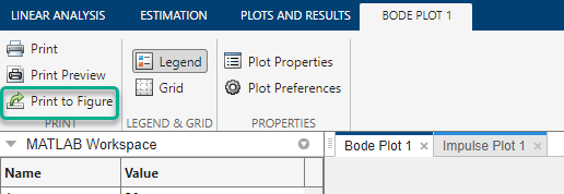
Select the plot you want to export. A tab appears with the same name as the plot.
Click the new tab. In the Print section, click Print to Figure.
A MATLAB figure window opens containing the plot.