Describing Function Analysis of Nonlinear Simulink Models

Describing function analysis is a technique for studying the frequency response of nonlinear systems. It is an extension of linear frequency response analysis. In linear systems, transfer functions depend only on the frequency of the input signal. In nonlinear systems, when a specific class of input signal, such as a sinusoid, is applied to a nonlinear element, you can represent the nonlinear element using a describing function. A describing function depends not only on the input frequency but also on the input amplitude. Describing function analysis has a wide area of applications from frequency response analysis to the prediction of limit cycles.

To use sinusoidal-input describing function analysis, which is the most common type of describing function analysis, your model should satisfy the following conditions.

In this example, you perform describing function analysis on a model with a saturation nonlinearity that satisfies these conditions.

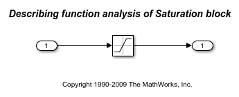
Open the Simulink® model.

mdl = 'scdsaturationDF';
open_system(mdl)

The saturation nonlinearity has the following sinusoidal input describing function.

Here, for a saturation with upper and lower limits of 0.5 and -0.5, respectively, and A is the amplitude of the sinusoidal input signal.

Compute and plot the describing function for amplitudes varying between 0.1 and 2.1. The describing function is implemented in saturationDF.m.

A = linspace(0.1,2.1,21);
N_A = saturationDF(0.5./A);
plot(A, N_A)
xlabel('Amplitude')
ylabel('N_A(A)')
title('Describing Function for Saturation')

You can compute the describing function for the saturation nonlinearity using frestimate over the same set of amplitudes for a fixed frequency of 5 rad/s. Since the describing function for a saturation does not depend on frequency, it is sufficient to run the analysis at a single frequency.

Define the input and output linear analysis points.

io(1) = linio('scdsaturationDF/In1',1,'input');
io(2) = linio('scdsaturationDF/Saturation',1,'output');

For each amplitude, create a sinestream input with the fixed 5 rad/s frequency and given amplitude. Then, run frestimate using this input signal.

w = 5;
N_A_withfrest = zeros(size(N_A));
for ct = 1:numel(A)
    in = frest.Sinestream('Frequency',w,'Amplitude',A(ct));
    sysest = frestimate(mdl,in,io);
    N_A_withfrest(ct) = real(sysest.resp);
end

Plot the frequency response estimation result along with the describing function.

plot(A,N_A,A,N_A_withfrest,'r*')
xlabel('Amplitude')
ylabel('N_A(A)')
title('Describing Function for Saturation Using frestimate')
legend('Describing function','Frequency response estimate')

Close the model.

bdclose(mdl)

You can also run a closed-loop describing function analysis over a frequency range. Open the model for this analysis.

mdl = 'scdsaturationDFcl';
open_system(mdl)

To begin, analytically compute the frequency response from the reference to the output using describing functions. To do so, first compute the amplitude of the input signal to the nonlinearity, given the reference amplitude and frequency. The input amplitude for the nonlinearity is not necessarily equal to the reference amplitude.

L = zpk([],[0 -1 -10],1);
w = logspace(-2,2,50);
A_DF = zeros(numel(A),numel(w));
for ct_amp = 1:numel(A)
    for ct_freq = 1:numel(w)
        % Compute the input amplitude to the nonlinearity by solving the
        % analytical equation.
        opt = optimset('Display','off');
        A_DF(ct_amp,ct_freq) = ...
            fzero(@(A_DF) solveForSatAmp(A_DF,L,w(ct_freq),A(ct_amp)),...
            A(ct_amp),opt);
    end
end

Next, for each amplitude, compute the analytical frequency response of the closed-loop system from the reference to the output using the describing function. Store the results in an array of frd objects.

L_w = freqresp(L,w);
for ct = 1:numel(A)
    N_A = saturationDF(0.5./A_DF(ct,:));
    cl_resp = N_A(:).*L_w(:)./(1+N_A(:).*L_w(:));
    cl(1,1,ct) = frd(cl_resp,w);
end

Obtain the frequency response for the closed-loop system using frestimate in a manner similar to the saturation describing function analysis.

io(1) = linio('scdsaturationDFcl/r',1,'input');
io(2) = linio('scdsaturationDFcl/Linear',1,'output');
for ct = 1:numel(A)
    in = frest.Sinestream('Frequency',w,'Amplitude',A(ct),...
        'NumPeriods',10,'SettlingPeriods',7);
    cl_withfrest(1,1,ct)  = frestimate(mdl,in,io);
end

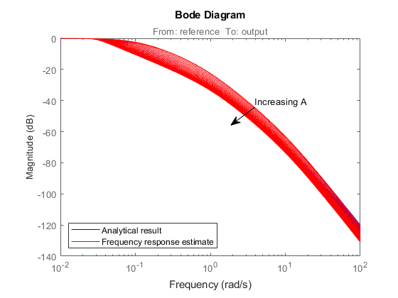
Plot the analytically calculated closed-loop magnitude along with the result from frestimate. As expected, the results match. The arrow indicates the direction of increasing amplitude.

h = figure;
bodemag(cl,'b',cl_withfrest,'r')
annotation(h,'textarrow',[0.64 0.58],[0.64 0.58],'String','Increasing A');
legend('Analytical result','Frequency response estimate',...
    'Location','southwest')

Close the model.

bdclose(mdl)