Electric Power Steering Controller Tuning Using systune
R2026bThis example demonstrates how to design and tune a linear compensator for an electric power steering (EPS) system using the systune function.
Electric power steering systems use an electric motor to provide steering assist torque to the driver. The controller must ensure that the steering feel is natural and responsive while rejecting road disturbances and maintaining stability across operating conditions.
EPS System Overview
An EPS system consists of the following key components:
Steering column and wheel: Connected to the driver, with inertia J1 and damping C1.
Rack and pinion mechanism: Converts rotational motion to linear motion at the wheels, with inertia J2 and damping C2.
Torsion bar: Connects the steering column to the rack with stiffness K. The torsion bar deflection is measured by a torque sensor.
Electric motor: Provides assist torque (Tau_a) to reduce driver effort.
Torque sensor: Measures the torsion bar torque (Tau_s) which is proportional to the angular difference between the steering column and the rack.
The control objective is to amplify input torque from drivers so that minimal effort is required to steer the vehicle, while maintaining good steering feel and stability.
Plant Model Parameters
Define the mechanical parameters of the EPS system. These values represent a typical column-assist EPS configuration.
K = 143.24; % Nm/rad
J1 = 0.044; % kg.m^2
C1 = 0.25; % Nm.s/rad
J2 = 0.11; % kg.m^2
C2 = 1.35; % Nm.s/rad
wm = 100; % Hz
Torque Map and Assist Curve Parameters
The torque map defines the relationship between measured torsion bar torque and the desired assist torque. In a production EPS system, this is typically a nonlinear lookup table (assist curve). For linear analysis, we use a linear gain approximation around the operating point.
The assist gain Kv determines how much the motor amplifies the driver torque. Higher values provide lighter steering feel but may reduce road feedback and stability margins.
Kv = 35;
Tau_s0 = 2; % Nm
Tau_friction = 2; % Nm
Compensator Structure Selection
The EPS compensator shapes the frequency response of the assist loop to achieve several objectives:
Low frequency: High gain to provide adequate assist and reduce driver effort.
Crossover region: Controlled roll-off with sufficient phase margin to ensure smooth, stable response.
High frequency: Attenuation to reject sensor noise and avoid excitation of structural resonances.
The compensator is typically implemented as a cascade of lead-lag filters. Here we show four progressively more complex designs:
Case 1: Single lead filter (basic phase boost)
Case 2: Single lead filter with higher bandwidth
Case 3: Two lead-lag stages for more phase margin
Case 4: Three lead-lag stages (highest performance baseline)
ControllerChoice = 4;

switch ControllerChoice
    case 1
        Gl1 = tf([1/100 1],[1/150 1]);
        Gl2 = tf(1,1);
        Gl3 = tf(1,1);
    case 2
        Gl1 = tf([1/100 1],[1/300 1]);
        Gl2 = tf(1,1);
        Gl3 = tf(1,1);
    case 3
        Gl1 = tf([1/100 1],[1/300 1]);
        Gl2 = tf([1/25 1],[1/5 1]);
        Gl3 = tf(1,1);
    case 4
        Gl1 = tf([1/55.3 1],[1/1000 1]);
        Gl2 = tf([1/32.7 1],[1/6 1]);
        Gl3 = tf([1/80.2 1],[1/713 1]);
end
Linearize the EPS Plant Model
Linearize the Simulink model to extract the transfer function from motor assist torque (Tau_a) to torsion bar torque (Tau_s). This captures the coupled dynamics of the steering column and rack through the torsion bar.
mdl_CST = "EPS_linear_simple_CST_Tuning";
open_system(mdl_CST);
The linearization points are configured to:
Opens the loop at the motor input to inject the assist torque signal.
Measures the torsion bar torque at the sensor output.
Breaks the driver torque and road disturbance paths to isolate the assist control loop for single-loop analysis.
io_s_a(1) = linio(strcat(mdl_CST,"/Motor System"),1,"openinput");
io_s_a(2) = linio(strcat(mdl_CST,"/Gain"),1,"output");
io_s_a(3) = linio(strcat(mdl_CST,"/Driver Torque Command"),1,"loopbreak");
io_s_a(4) = linio(strcat(mdl_CST,"/Road Disturbance"),1,"loopbreak");
Linearize the Simulink model at the model initial condition. Rename the linearization result as Peq in subsequent controller design tasks.
linsys_s_a = linearize(mdl_CST,io_s_a,0);
Peq = linsys_s_a;
Validate the Linearized Plant
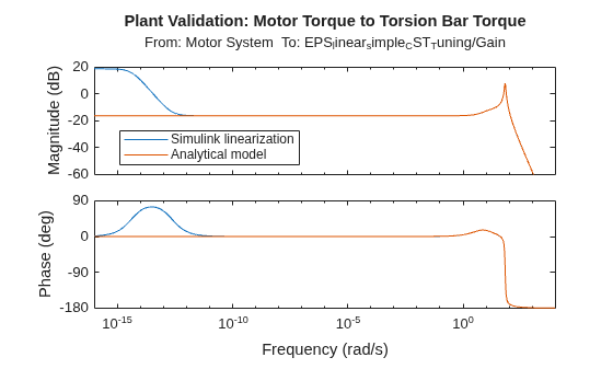
Compare the Simulink linearization against the analytical transfer function for the EPS system [1]. This validates that the Simulink model is correctly configured and the linearization points are correct.
figure
bodeplot(Peq,tf(K*[J1 C1 0],[J1*J2 J1*C2+J2*C1 C1*C2+J1*K+J2*K C1*K+C2*K 0]));
legend("Simulink linearization","Analytical model",...
        Location="best")
title("Plant Validation: Motor Torque to Torsion Bar Torque")
Construct the Closed-Loop System for Tuning
Assemble the feedback loop using named signal connections. The loop structure is:

Where:
Kv is the torque map gain (amplifies error signal)
C is the compensator (to be tuned)
Gm is the motor actuator dynamics (first-order lag)
Plant maps motor torque to torsion bar torque
Peq.InputName = "Tau_a";
Peq.OutputName = "Tau_s_neg";

Gain_TorqueMap = tf(Kv*1,1);
Gain_TorqueMap.InputName = "Tau_s";
Gain_TorqueMap.OutputName = "ctrl_input";

Gm = tf(wm,[1 wm]);
Gm.InputName = "Tau_a_ref";
Gm.OutputName = "Tau_a";
Define the Tunable Compensator
Use tunableTF to create a parametric transfer function that systune will optimize. We choose a 2nd-order compensator (2 zeros, 2 poles) as a good balance between performance and implementation complexity.
The minimum coefficient constraints ensure that the tuned compensator remains minimum-phase and stable (all coefficients positive), which guarantees a realizable controller.
C = tunableTF('controller',2,2);
C.Numerator.Minimum = ones(1,3);
C.Denominator.Minimum = ones(1,3);
C.InputName = "ctrl_input";
C.OutputName = "Tau_a_ref";
Connect the System and Define Analysis Points
Form the closed-loop system with analysis points at key locations for evaluating loop transfer, margins, and sensitivity.
sum_Tau = sumblk("Tau_s = Tau_ref - Tau_s_neg");

input = {"Tau_ref"};
output = {"Tau_s_neg"};
APs = {"ctrl_input","Tau_a_ref","Tau_a","Tau_s_neg"};

ST0 = connect(Peq,Gain_TorqueMap,C,Gm,sum_Tau,input,output,APs)
ST0 =
Generalized continuous-time state-space model with 1 outputs, 1 inputs, 7 states, and the following blocks:
  CONNECT_AP1: Analysis point, 4 channels, 1 occurrences.
  controller: Tunable SISO transfer function, 2 zeros, 2 poles, 1 occurrences.
Model Properties

Type "ss(ST0)" to see the current value and "ST0.Blocks" to interact with the blocks.
Define Tuning Goals
The tuning goals encode the frequency-domain performance requirements:
Loop Shape Goal (LS1): Target crossover frequency of 200 rad/s. This defines the assist bandwidth — the frequency up to which the motor actively assists the driver. A 200 rad/s bandwidth (~32 Hz) provides responsive steering without amplifying high-frequency noise from the torque sensor or road surface roughness.
Margins Goal (MG1): At least 3 dB gain margin and 45 degrees phase margin, enforced in the 100-3000 rad/s frequency range. These margins are critical for EPS because:
Vehicle parameters vary with speed, load, and tire conditions
Temperature affects motor resistance and torsion bar stiffness
Manufacturing tolerances create unit-to-unit variation
Insufficient phase margin causes steering oscillations perceived as "shimmy" or "nibble" by the driver
LS1 = TuningGoal.LoopShape("Tau_s_neg",200);
MG1 = TuningGoal.Margins("Tau_s_neg",3,45);
MG1.Focus = [100 3000];
Configure and Run systune
systune uses nonsmooth optimization to jointly satisfy all tuning goals. Key options:
RandomStart=5: Run 5 random restarts to increase confidence in finding a global optimum. The EPS tuning landscape may have local minima due to the interaction between gain and phase constraints.SoftTol: Convergence tolerance for soft goals.MinDecay: Minimum closed-loop pole decay rate.MaxRadius: Maximum closed-loop pole magnitude.
All goals are specified as soft constraints. The optimizer minimizes the worst-case violation across all goals. A final soft value <= 1 means all goals are satisfied; values > 1 indicate the degree of violation.
opt = systuneOptions(SoftTol = 1e-10,...
                    MinDecay = 1e-10,...
                    MaxRadius = 1e10,...
                    RandomStart = 5);
rng(1);
warning("off","Control:tuning:TuningWarning1");
[ST1,fSoft,fHard] = systune(ST0,[LS1,MG1],[],opt);
Final: Soft = 2.1, Hard = -Inf, Iterations = 90
Final: Soft = 2.63, Hard = -Inf, Iterations = 89
Final: Soft = 2.31, Hard = -Inf, Iterations = 148
Final: Soft = 2.41, Hard = -Inf, Iterations = 87
Final: Soft = 2.15, Hard = -Inf, Iterations = 201
Final: Soft = 2.34, Hard = -Inf, Iterations = 99
Recover the warning state after tuning.
warning("on","Control:tuning:TuningWarning1");
Evaluate Goal Satisfaction
Visualize how well the tuned PID design meets each requirement. The shaded regions indicate violation of the respective goal.
figure
viewGoal(LS1,ST1);
title("Loop Shape Goal: Target Crossover at 200 rad/s")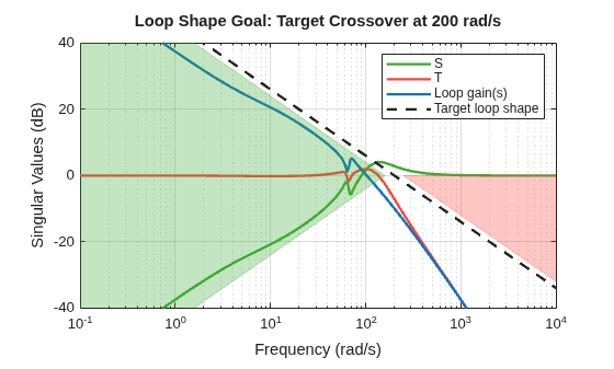
figure;
viewGoal(MG1,ST1);
title("Margins Goal: GM >= 3 dB, PM >= 45 deg in [100, 3000] rad/s");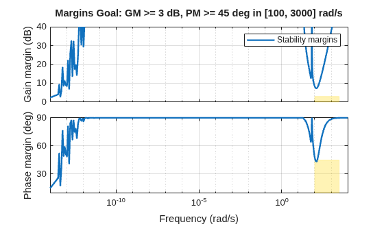
Extract and Analyze the Tuned Controller
Retrieve the optimized compensator transfer function and verify the resulting loop transfer function meets the stability margin requirements.
C_Tuned = getBlockValue(ST1).controller;
disp("Tuned compensator transfer function:");
Tuned compensator transfer function:
C_Tuned
C_Tuned =
  8.397 s^2 + 45.73 s + 3.627e04
  ------------------------------
       s^2 + 2685 s + 2.82

Name: controller
Continuous-time transfer function.
Model Properties
Verify Stability Margins
Compute the open-loop transfer function (loop broken at the plant output) and display the Bode plot with gain and phase margins annotated.
For EPS applications, typical requirements are:
Gain margin >= 6 dB (to handle assist gain variations)
Phase margin >= 45 degrees (to prevent oscillations)
Crossover frequency between 100-300 rad/s (for responsive feel)
LoopTransfer = Gain_TorqueMap*C_Tuned*Gm*Peq;
figure;
margin(LoopTransfer);
title("Open-Loop Transfer Function with Stability Margins");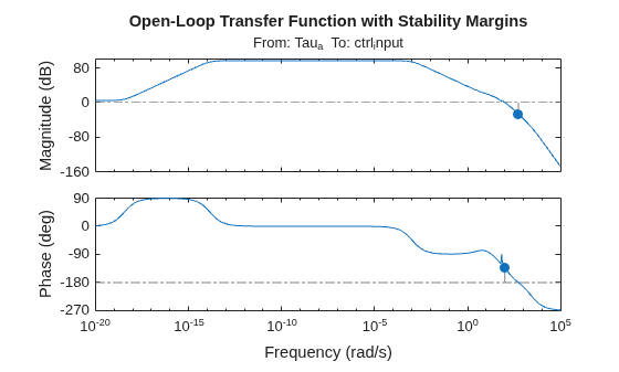
Simulate and Compare Controller Performance
Compare the tuned compensator against the baseline lead-lag design in a time-domain simulation. The test scenario applies a representative driver torque input and evaluates:
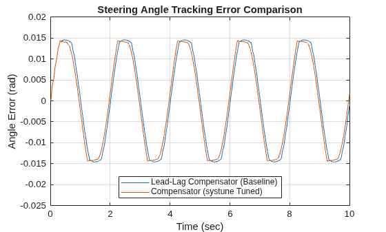
Steering angle tracking error: Measures how precisely the rack follows driver intent. Lower error means more responsive, predictable steering.
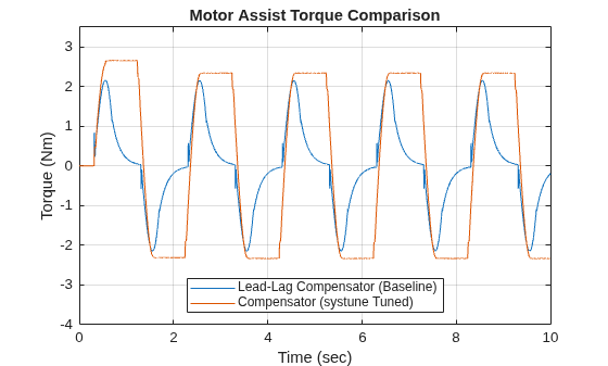
Motor assist torque profile: Indicates control effort and smoothness. Abrupt torque changes cause audible motor whine and tactile vibration at the steering wheel.
mdl_compare_ctrl = "EPS_linear_simple_CompareControl";
open_system(mdl_compare_ctrl);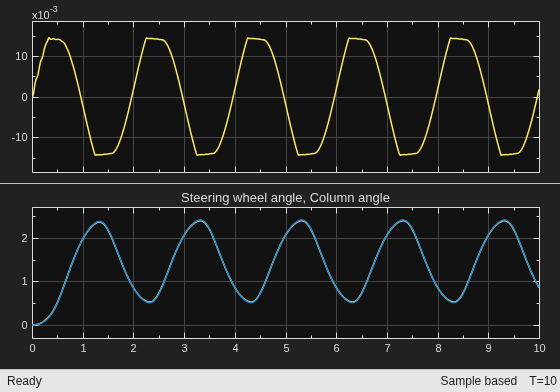
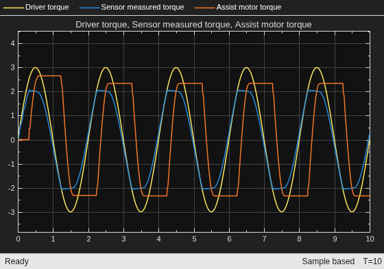
Use the bench mark lead-lag compensator for initial simulation result.
controller_implementation = ...
    strcat(mdl_compare_ctrl,"/Controller/Controller Implementation");
set_param(controller_implementation,"LabelModeActiveChoice","LeadLagComp");
simOutLeadLagComp = sim(mdl_compare_ctrl);
Time_LeadLagComp = simOutLeadLagComp.tout;
Tau_a_LeadLagComp = simOutLeadLagComp.TorqueComparisonScope.signals(3).values;
Angle_error_LeadLagComp = simOutLeadLagComp.AngleComparisonScope.signals(1).values;
Change the active choice to tuned compensator.
set_param(strcat(controller_implementation,"/Lead-Lag Compensator/LTI System"),"sys","C_Tuned");
simOutCompTuned = sim(mdl_compare_ctrl);
Time_CompTuned = simOutCompTuned.tout;
Tau_a_CompTuned = simOutCompTuned.TorqueComparisonScope.signals(3).values;
Angle_error_CompTuned = simOutCompTuned.AngleComparisonScope.signals(1).values;
Plot Performance Comparison
Compare steering angle tracking error and motor torque between the two controller architectures.
figure
plot(Time_LeadLagComp, Angle_error_LeadLagComp)
hold on
plot(Time_CompTuned, Angle_error_CompTuned)
ylim([-0.025 0.02])
xlabel("Time (sec)")
ylabel("Angle Error (rad)")
title("Steering Angle Tracking Error Comparison")
legend("Lead-Lag Compensator (Baseline)","Compensator (systune Tuned)", ...
        Location = "south")
grid on
figure
plot(Time_LeadLagComp, Tau_a_LeadLagComp)
hold on
plot(Time_CompTuned, Tau_a_CompTuned)
ylim([-4 3.5])
xlabel("Time (sec)")
ylabel("Torque (Nm)")
title("Motor Assist Torque Comparison")
legend("Lead-Lag Compensator (Baseline)","Compensator (systune Tuned)", ...
        Location = "south")
grid on
Summary
This example demonstrates multi-stage compensator tuning for EPS using systune. The workflow consists of:
Define plant parameters from the EPS mechanical system.
Linearize the Simulink model to obtain the assist loop plant.
Specify a tunable compensator structure using
tunableTF.Encode performance requirements as
TuningGoalobjects.Optimize compensator parameters with
systuneusing multiple random starts.Validate in both frequency domain (margins) and time domain (simulation).
References
[1] Lee, D., Kim, K. S., & Kim, S. (2017). Controller design of an electric power steering system. IEEE Transactions on Control Systems Technology, 26(2), 748-755.

