Identify Frequency Domain Features Using Frequency Response Estimator Block

Linearize Model

Open the Simulink® model for the lightweight airplane. For more information on this model, see Lightweight Airplane Design (Aerospace Blockset).

mdl = 'scdskyhoggOnlineFRE';
open_system(mdl)

Linearize the lightweight airplane model from the altitude command signal, AltCmd, to the sensed height, h_sensed. These linear analysis points are already specified in the model.

io = getlinio(mdl)

2x1 vector of Linearization IOs: 
--------------------------
1. Linearization input perturbation located at the following signal:
- Block: scdskyhoggOnlineFRE/Pilot/Frequency Response Estimator
- Port: 1
- Signal Name: AltCmd
2. Linearization output measurement located at the following signal:
- Block: scdskyhoggOnlineFRE/Vehicle System Model/Avionics/Autopilot/Bus Selector1
- Port: 1
- Signal Name: <h_sensed>

To linearize the model, use the linearize function. The model is preconfigured to use an operating point obtained using a simulation snapshot at t = 75.

sys = linearize(mdl,io);

Plot the Bode response of the linearized model.

bode(sys)
hold on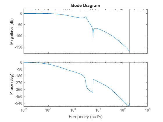

The linearization result captures characteristics of the nonlinear model, such as the antiresonance around 6.28 rad/s.

Estimate Frequency Response Using Frequency Response Estimator

Traditional experiment modes, such as sinestream and superposition, are generally sufficient for frequency response estimation purposes. To capture the frequency response over a range, you can create a frequency vector using logspace. For example, the command logspace(-1,1,6) generates six frequency points between 0.1 rad/s and 10 rad/s.

In the scdskyhoggOnlineFRE model, the Frequency Response Estimator block is configured as follows.

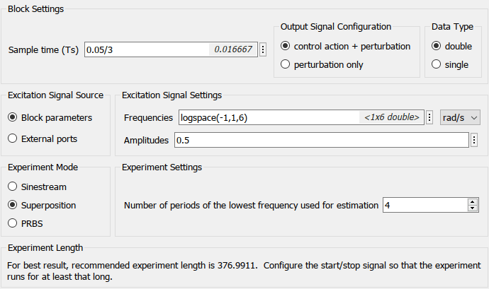
The block recommends an experiment length of 377 s. This this the length required to obtain an accurate estimation result. The model is already configured to run for 385 s.

Simulate the model to obtain the frequency response result with superposition experiment mode.

sim(mdl);
sys_estim_superposition = frd(frdata,logspace(-1,1,6));
bode(sys_estim_superposition,'r*')

The antiresonance around 6.28 rad/s is missing from the coarse frequency points. To capture the feature, you can increase the number of frequency points, from six to 24.

Run the estimation and plot the frequency response.

set_param([mdl,'/Pilot/Frequency Response Estimator'],'Frequencies','logspace(-1,1,24)');
sim(mdl);
sys_estim_superposition = frd(frdata,logspace(-1,1,24));
bode(sys_estim_superposition,'ro')
legend('Linearization result','FRE (6 points)','FRE (24 points)')
hold off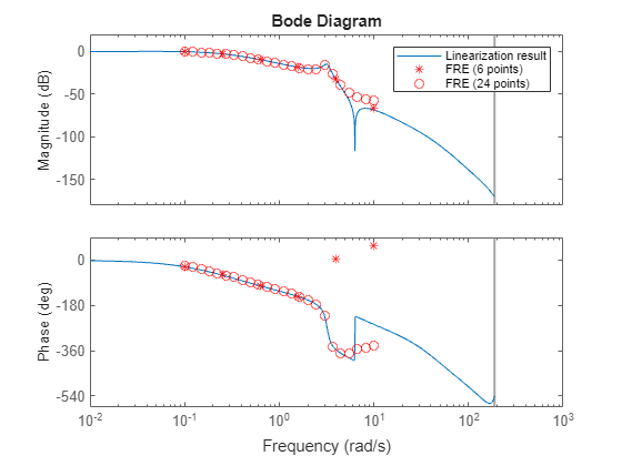

Simply increasing the number does not lead to more accurate result, as the discrepancy from linearization result increases. Another alternative is to use the sinestream experiment mode, but that will require a much longer experiment length. For instance, keeping the 24 frequency points in between 0.1 rad/s and 10 rad/s requires an experiment length of more than 2060 s.

Use PRBS Experiment Mode to Save Experiment Time

To use PRBS input signal, set the experiment mode to PRBS. The block dialog recommends the values for PRBS parameters based on the specified frequencies. For this example, the block recommends number of periods as 3 and signal order as 13. You can use the autogenerated values, but to keep the experiment time minimum, use 1 as the number of periods. This configuration requires an experiment length of 136.5 s.

Set the block parameters.

set_param([mdl,'/Pilot/Frequency Response Estimator'],'Frequencies','logspace(-1,1,24)');
set_param([mdl,'/Pilot/Frequency Response Estimator'],'ExperimentMode','PRBS');
set_param([mdl,'/Pilot/Frequency Response Estimator'],'Amplitudes','0.25');
set_param([mdl,'/stop'],'Time','142');
set_param(mdl,'StopTime','145');

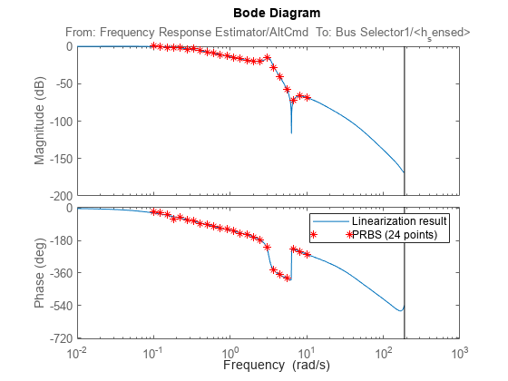
Run the estimation and compare the analytical linearization result against the online frequency response estimation result.

figure
sim(mdl);
sys_estim_PRBS = frd(frdata,logspace(-1,1,24));
bode(sys,sys_estim_PRBS,'r*')
legend('Linearization result','PRBS (24 points)')

The frequency response data and analytical linearization result match well.

Without an analytical LTI model, such as a transfer function, it is impossible to know where to investigate in frequency domain. With much shorter experiment time, the PRBS experiment mode achieves a more accurate frequency response estimation result, and provides an indication of the antiresonance. Based on this indication, you can investigate the system further over a much narrower frequency range. Using the PRBS mode, you can obtain a frequency response with much higher resolution from an experiment with the same length. The PRBS experiment mode is a powerful tool for running frequency response estimation experiments, especially when dealing with a nonlinear system with interesting frequency domain characteristics.

Close the model.

close_system(mdl,0)