Modal Analysis of IEEE 9-Bus System Model Using Linearization

Power System Modal Analysis

Power system modal analysis is a fundamental technique for assessing the dynamic stability of interconnected power networks. In large-scale grids, generators interact through the transmission network, and their coupled electromechanical dynamics give rise to oscillatory modes.

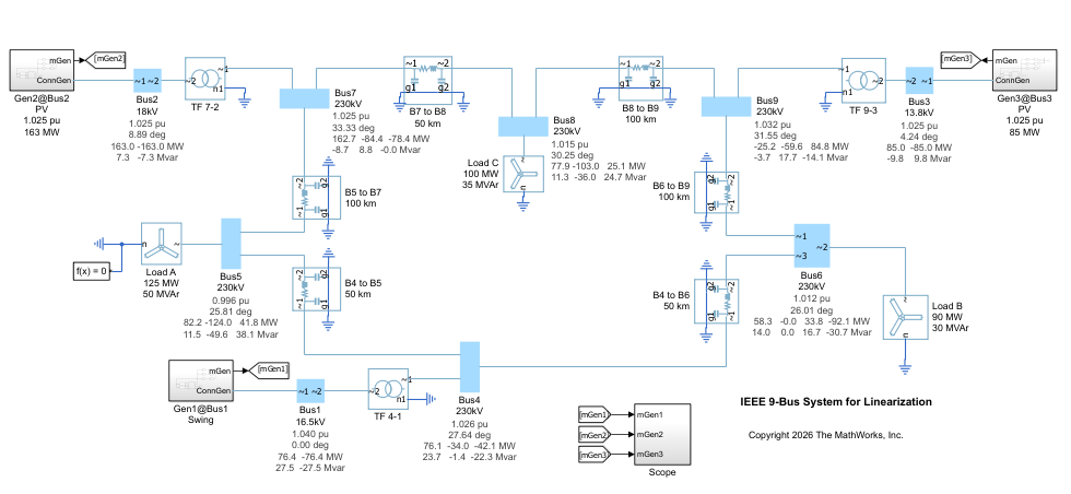
The IEEE 9-bus system is a benchmark model consisting of three generators, three loads, and nine buses connected via transmission lines. It exhibits both local and inter-area oscillation modes, making it ideal for demonstrating modal analysis techniques. The IEEE 9-bus system IEEE 9-Bus System (Simscape Electrical) is modeled using Simscape Electrical, capturing all dynamics mentioned above. In addition, the Simulink model is linearizable, enabling smooth modal analysis workflows.

Linearize the IEEE 9-Bus System Model

Open the Simulink model configured for linearization. This model has linearization I/O points pre-configured: the inputs are perturbations to mechanical power at each generator, and the outputs are frequency deviations measured at each generator terminal.

mdl = "IEEE9BusSystemLinearization";
open_system(mdl);

For synchronous generators, input is the torque Tm in the Governor and Prime Mover subsystems and the voltage Vref in the AVR and Exciter subsystems.

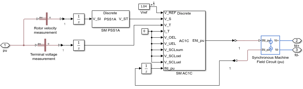
Outputs are the rotor speed, that is frequency, and terminal voltage of the machine from the Scope subsystem.

Perform Linearization

Linearize at t = 6 sec when the system has reached steady state. The linearize function computes the state-space model between the selected I/O points. The getlinio function retrieves the linear analysis points saved in the model. Before linearization, suppress warning messages for simulation purposes.

warning("off","Simulink:blocks:BmathSqrtOfNegativeNumber");
[linsys,~] = linearize(mdl,getlinio(mdl),6);

Linearization result linsys is a 6-by-6 state-space LTI model, according to the linear analysis point specifications.

Debug Linearization Result

Before conducting modal analysis, you need to review diagnostic information about individual block linearization. Some blocks in a Simulink model may linearize to zero because of its implementation. You can debug this linearization-to-zero behavior using the Linearization Advisor. For more information, see Troubleshoot Linearization Results at Command Line or Troubleshoot Linearization Results in Model Linearizer.

Using Linearization Advisor, you can find that the Voltage Transducer in the SM AC1C (Simscape Electrical) block linearizes to zero.

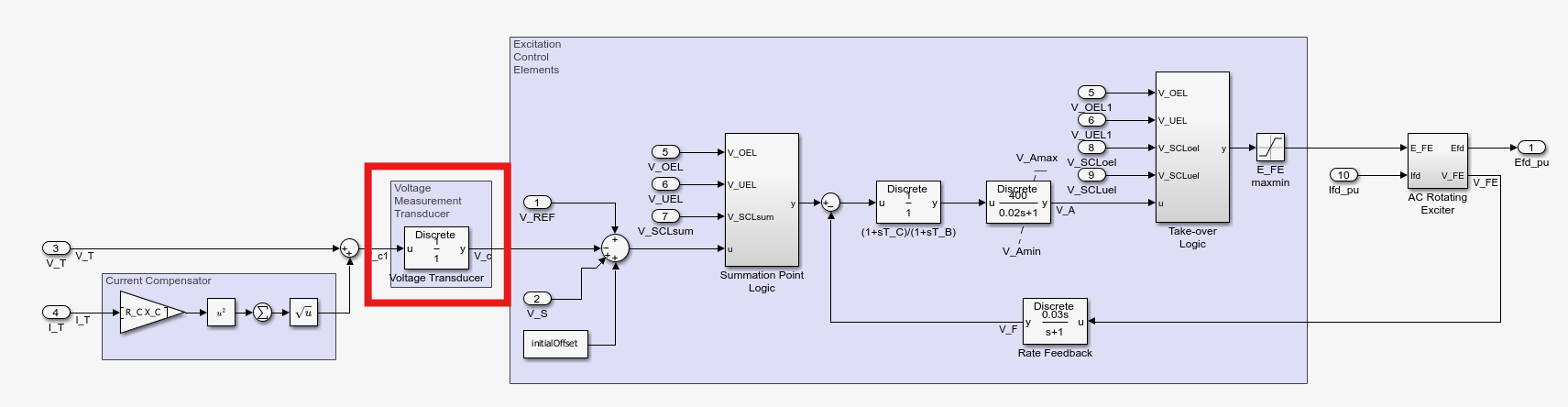
To verify this behavior, you can linearize only the block at the snapshot time of 6 sec.

SMblkio = strcat(mdl,"/Gen1@Bus1 Swing/AVR and Exciter/SM AC1C/Voltage Transducer");
SMblksys = linearize(mdl,SMblkio,6)

SMblksys = 
  D = 
                 Voltage Tran
   Voltage Tran             0
 
Static gain.
Model Properties

Correct Linearization Result

You can correct the linearization result using block substitution for the Voltage Transducer blocks. Before commenting out the blocks, turn off the warning about modifying parameters inside a library link.

warning("off","Simulink:Commands:SetParamLinkChangeWarn");
SMVTGen1 = strcat(mdl,"/Gen1@Bus1 Swing/AVR and Exciter/SM AC1C/Voltage Transducer");
SMVTGen2 = strcat(mdl,"/Gen2@Bus2 PV 1.025 pu 163 MW/AVR and Exciter/SM AC1C/Voltage Transducer");
SMVTGen3 = strcat(mdl,"/Gen3@Bus3 PV 1.025 pu 85 MW/AVR and Exciter/SM AC1C/Voltage Transducer");
set_param(SMVTGen1,"SCDEnableBlockLinearizationSpecification","on");
set_param(SMVTGen2,"SCDEnableBlockLinearizationSpecification","on");
set_param(SMVTGen3,"SCDEnableBlockLinearizationSpecification","on");
rep = struct("Specification",'tf(1,1,Ts)',...
    "Type",'Expression',...
    "ParameterNames",'',...
    "ParameterValues",'');
set_param(SMVTGen1,"SCDBlockLinearizationSpecification",rep);
set_param(SMVTGen2,"SCDBlockLinearizationSpecification",rep);
set_param(SMVTGen3,"SCDBlockLinearizationSpecification",rep);
[linsys,linop] = linearize(mdl,getlinio(mdl),6);

Check Stability of Linearized Model

Verify that all eigenvalues of the linearized system have negative real parts, confirming small-signal stability at the operating point.

isstable(linsys)

ans = logical
   1

Simulate Time-Domain Response

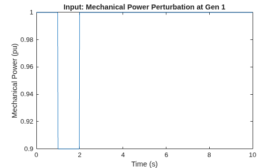
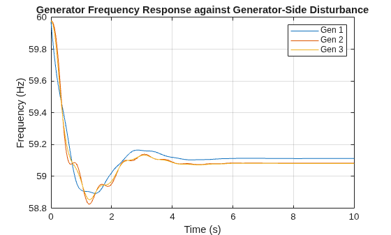
Examine the time-domain response of each generator against a step change in mechanical power of Generator 1: a 10% reduction at t = 1 sec lasting for 1 sec. This step change excites the electromechanical modes and reveals oscillatory behavior.

Ts = linsys.Ts;
[u, t] = gensig("square", 2, 10, Ts);
u(121:end) = 0;
u_G1 = 1 - 0.1*u;
figure
plot(t, u_G1)
xlabel("Time (s)")
ylabel("Mechanical Power (pu)")
title("Input: Mechanical Power Perturbation at Gen 1")

Compute Generator Time-Domain Responses Using Linearized Model

Extract single-input single-output (SISO) subsystems from the MIMO linearized model. Each subsystem represents the transfer function from Gen 1 mechanical power to frequency deviation at Gen 1, Gen 2, and Gen 3.

sysG1toG1 = linsys(1,2);
sysG1toG2 = linsys(2,2);
sysG1toG3 = linsys(3,2);

Find initial conditions consistent with the DC operating point and obtain time-domain simulation curves. The input is a 10% reduction from the nominal generator output of 0.31233 p.u. at Gen1.

opG1toG1 = findop(sysG1toG1, y=dcgain(sysG1toG1));
yG1 = lsim(sysG1toG1, u_G1*0.31233, t, opG1toG1);

opG1toG2 = findop(sysG1toG2, y=dcgain(sysG1toG2));
yG2 = lsim(sysG1toG2, u_G1*0.31233, t, opG1toG2);

opG1toG3 = findop(sysG1toG3, y=dcgain(sysG1toG3));
yG3 = lsim(sysG1toG3, u_G1*0.31233, t, opG1toG3);

Plot the frequency at each generator bus. The oscillatory behavior reveals the electromechanical modes excited by the disturbance. Observe that generators oscillate against each other at the inter-area mode frequency.

figure
plot(t, 60*(1+yG1), t, 60*(1+yG2), t, 60*(1+yG3))
xlabel("Time (s)")
ylabel("Frequency (Hz)")
title("Generator Frequency Response against Generator-Side Disturbance")
legend("Gen 1", "Gen 2", "Gen 3")
grid on

Modal Analysis Using Linear Model

Use modalsep to decompose the MIMO system into a parallel connection of individual modal subsystems. Each modal subsystem corresponds to a pair of complex-conjugate eigenvalues (or a real eigenvalue). The number of modal subsystems equals the number of distinct modes.

[H, H0] = modalsep(linsys);
numModes = size(H, 3);
disp("Number of modal subsystems: " + numModes)

Number of modal subsystems: 66

Extract Mode Frequencies and Damping Ratios

Use damp to compute the natural frequency and damping ratio of each pole. These characterize the oscillatory behavior: frequency determines the oscillation rate, and damping ratio determines how fast the oscillation decays.

[Wn, Zeta, P] = damp(linsys);
All_modes = [Wn/(2*pi), Zeta];
disp("All modes [Frequency (Hz), Damping Ratio]:")

All modes [Frequency (Hz), Damping Ratio]:

disp(All_modes);

    0.0000    1.0000
    0.1491    0.6649
    0.1491    0.6649
    0.2118    1.0000
    0.2327    0.8060
    0.2327    0.8060
    0.3335    0.4865
    0.3335    0.4865
    0.4532    1.0000
    0.5183    1.0000
    0.7087    0.8327
    0.7087    0.8327
    1.0126    1.0000
    1.2416    1.0000
    1.2963    1.0000
    1.3893    0.1011
    1.3893    0.1011
    1.4912    1.0000
    1.7151    1.0000
    1.7151    1.0000
    2.1176    0.2027
    2.1176    0.2027
    2.4548    1.0000
    2.8373    1.0000
    3.5949    1.0000
    3.8837    1.0000
    5.8225    0.8052
    5.8225    0.8052
    5.9490    0.8081
    5.9490    0.8081
    6.1309    0.8082
    6.1309    0.8082
   28.4706    0.8799
   28.4706    0.8799
   32.0015    0.9098
   32.0015    0.9098
   42.1881    1.0000
   44.6656    1.0000
   45.4486    0.9523
   45.4486    0.9523
   58.9500    0.8608
  106.9640    1.0000
  107.5302    0.9603
  112.6432    0.9639
  121.6204    0.9914
  121.6204    0.9914
  123.3266    0.9973
  123.3266    0.9973
  125.6608    1.0000
  130.8573    1.0000
  132.5620    0.9830
  132.5620    0.9830
  136.9944    0.9864
  136.9944    0.9864
  138.7318    0.9969
  138.7318    0.9969
  146.7595    1.0000
  146.7615    1.0000
  148.3783    0.9941
  148.3783    0.9941
  158.1956    0.9983
  158.1956    0.9983
  160.5180    0.9824
  187.8723    1.0000
  199.0067    0.9886
  203.8376    0.9993
  203.8376    0.9993
  211.7523    1.0000
  215.9869    0.9925
  215.9869    0.9925
  223.4415    0.9990
  223.4415    0.9990
  228.8945    0.9964
  228.8945    0.9964
  231.6096    1.0000
  232.8078    0.9917
  233.3805    0.9994
  233.3805    0.9994
  240.8273    0.9996
  240.8273    0.9996
  249.5428    0.9927
  257.9566    1.0000
  258.2967    0.9932
  265.3396    1.0000
  265.3396    1.0000
  270.1777    1.0000
  270.2734    1.0000
  270.2995    1.0000
  272.7081    1.0000
  274.7112    0.9983
  274.7112    0.9983
  278.1390    1.0000
  353.9270    0.9964
  354.3158    1.0000
  371.9552    1.0000

Identify Critical Oscillatory Modes

Filter modes to identify those that are:

These criteria isolate the inter-area and local oscillation modes relevant to power system stability.

IX = find(Zeta < 0.2 & (Zeta > 0) & (Wn/(2*pi)) < 5);
ImportantModes = [Wn(IX)/(2*pi), Zeta(IX)];
disp("Important modes (f < 5 Hz, zeta < 0.2) [Frequency (Hz), Damping Ratio]:")

Important modes (f < 5 Hz, zeta < 0.2) [Frequency (Hz), Damping Ratio]:

disp(ImportantModes)

    1.3893    0.1011
    1.3893    0.1011

Impact of Power System Stabilizer Using Modal Analysis

For each synchronous generator, Power System Stabilizer (PSS) is added to the excitation system to damp electromechanical oscillations. A PSS typically uses signals like speed deviation or accelerating power to modulate the field voltage, creating damping torque to stabilize the power grid during disturbances.

In the IEEE 9-bus system, a SM PSS1A (Simscape Electrical) block implements a single-input PSS1A power system stabilizer (PSS) that maintains rotor angle stability in a synchronous machine (SM) in conformance with IEEE 421.5-2016 [1]. Typically, you use a PSS to enhance the damping of power system oscillations through excitation control.

The PSS blocks damp oscillations in the IEEE 9-bus system during simulation but they linearize to zero due to the implementation of the second-order low-pass filter blocks. To verify the PSS being linearized to zero in the small-signal model, you can linearize only the SM PSS1A block in the AVR and Exciter subsystem of each synchronous machine.

blkio = strcat(mdl,"/Gen1@Bus1 Swing/AVR and Exciter/SM PSS1A");
PSSblksys = linearize(mdl,blkio,6)

PSSblksys = 
  D = 
               SM PSS1A/1
   SM PSS1A/1           0
 
Static gain.
Model Properties

This zero linearization result directly leads to the important mode below 5 Hz that has a damping ratio of less than 0.2.

Obtain Correct Linearization Result of PSS Block

To obtain correct linearization result, comment through the low-pass filter and the lead-lag compensator blocks.

set_param(strcat(blkio,"/Second-Order Low-Pass Filter"),"commented","through");
set_param(strcat(blkio,"/Lead-Lag"),"commented","through");

Linearize the SM PSS1A block again at the same snapshot time at 6 sec.

PSSblklinsysSub = linearize(mdl,blkio,6);

After obtaining a valid linearization result, uncomment both blocks to recover the model to its original state.

set_param(strcat(blkio,"/Second-Order Low-Pass Filter"),"commented","off");
set_param(strcat(blkio,"/Lead-Lag"),"commented","off");

Resolve Linearization Issues Using Block Substitution

Using the valid PSS linearization result, you can specify the linearization of each SM PSS1A block without having to replace this block in the original IEEE 9-bus system model.

PSSGen1 = strcat(mdl,"/Gen1@Bus1 Swing/AVR and Exciter/SM PSS1A");
PSSGen2 = strcat(mdl,"/Gen2@Bus2 PV 1.025 pu 163 MW/AVR and Exciter/SM PSS1A");
PSSGen3 = strcat(mdl,"/Gen3@Bus3 PV 1.025 pu 85 MW/AVR and Exciter/SM PSS1A");
set_param(PSSGen1,"SCDEnableBlockLinearizationSpecification","on");
set_param(PSSGen2,"SCDEnableBlockLinearizationSpecification","on");
set_param(PSSGen3,"SCDEnableBlockLinearizationSpecification","on");
rep = struct("Specification",'PSSblklinsysSub',...
    "Type",'Expression',...
    "ParameterNames",'',...
    "ParameterValues",'');
set_param(PSSGen1,"SCDBlockLinearizationSpecification",rep);
set_param(PSSGen2,"SCDBlockLinearizationSpecification",rep);
set_param(PSSGen3,"SCDBlockLinearizationSpecification",rep);

Linearize the model again with specified individual block linearization settings.

[linsysPSS,~] = linearize(mdl,getlinio(mdl),6);

After linearization, disable the specified block linearizations for each PSS block and Voltage Transducer blocks.

set_param(PSSGen1,"SCDEnableBlockLinearizationSpecification","off");
set_param(PSSGen2,"SCDEnableBlockLinearizationSpecification","off");
set_param(PSSGen3,"SCDEnableBlockLinearizationSpecification","off");
set_param(SMVTGen1,"SCDEnableBlockLinearizationSpecification","off");
set_param(SMVTGen2,"SCDEnableBlockLinearizationSpecification","off");
set_param(SMVTGen3,"SCDEnableBlockLinearizationSpecification","off");

After linearization, reenable the warning message settings.

warning("on","Simulink:Commands:SetParamLinkChangeWarn");
warning("on","Simulink:blocks:BmathSqrtOfNegativeNumber");

Modal Analysis with Power System Stabilizer

Conduct modal analysis using the linearization result that includes PSS blocks.

[WnPSS, ZetaPSS, ~] = damp(linsysPSS);
IXPSS = find(ZetaPSS < 0.2 & (ZetaPSS > 0) & (WnPSS/(2*pi)) < 5);
ImportantModesPSS = [WnPSS(IXPSS)/(2*pi), ZetaPSS(IXPSS)];
disp("Important modes (f < 5 Hz, zeta < 0.2) [Frequency (Hz), Damping Ratio]:")

Important modes (f < 5 Hz, zeta < 0.2) [Frequency (Hz), Damping Ratio]:

disp(ImportantModesPSS);

    1.4769    0.1156
    1.4769    0.1156
    2.2727    0.1523
    2.2727    0.1523

Compared to the important modes without PSS, the slowest mode becomes faster with a higher damping ratio. As a result, PSS blocks enhance the damping of power system oscillations through excitation control.

Using the same modal analysis approach, you can fine tune parameters inside the PSS to further improve the power system stability.

Summary

This example demonstrated power system oscillatory stability analysis. The linearization-based modal analysis workflow provides exact eigenvalues, damping ratios, and mode shapes. The linearization result accurately captures the small-signal dynamics of the IEEE 9-bus system. Furthermore, the impact of power system stabilizer is demonstrated using information obtained from modal analysis.

References

[1] “IEEE Recommended Practice for Excitation System Models for Power System Stability Studies.” IEEE Std 421.5-2016 (Revision of IEEE Std 421.5-2005), August 2016, 1–207. https://doi.org/10.1109/IEEESTD.2016.7553421.