Visualize Linear System of a Continuous-Time Model Discretized During Simulation
This example shows how to discretize a continuous-time model during simulation and plot the model's discretized linear behavior.
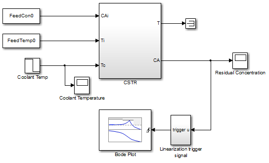
Open the Simulink® model:
scdcstr

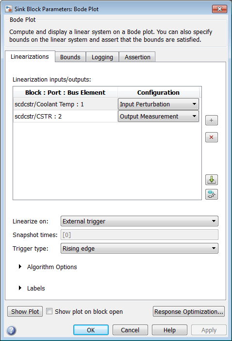
In this model, the Bode Plot block has already been configured with:
Input point at the coolant temperature input
Coolant
Temp
Output point at the residual concentration output
CASettings to linearize the model on a rising edge of an external trigger. The trigger signal is modeled in the
Linearization
trigger signal
block in the model.Saving the computed linear system in the MATLAB® workspace as
LinearReactor.
To view these configurations, double-click the block.

To learn more about the block parameters, see the block reference pages.
Specify the sample time to compute the discrete-time linear system.
Click
 adjacent to Algorithm Options.
The option expands to display the linearization algorithm options.

Specify a sample time of 2 in the Linear system sample time field.
To learn more about this option, see the block reference page.
Click Show Plot to open an empty Bode plot window.
Plot the Bode magnitude and phase by clicking
 in the plot window.
During simulation, the software:
Linearizes the model on encountering a rising edge.
Converts the continuous-time model into a discrete-time linear model with a sample time of 2. This conversion uses the default
Zero-Order
Hold
method to perform the sample time conversion.The software plots the discrete-time linear behavior in the Bode plot window. After the simulation completes, the plot window resembles the following figure.

The plot shows the Bode magnitude and phase up to the Nyquist frequency, which is computed using the specified sample time. The vertical line on the plot represents the Nyquist frequency.
See Also
Bode Plot | Gain and Phase Margin Plot | Linear Step Response Plot | Nichols Plot | Pole-Zero Plot | Singular Value Plot