How to Build a Multibody System in MATLAB

Problem Description

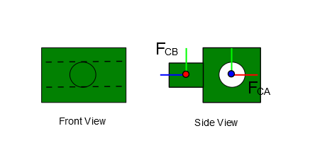
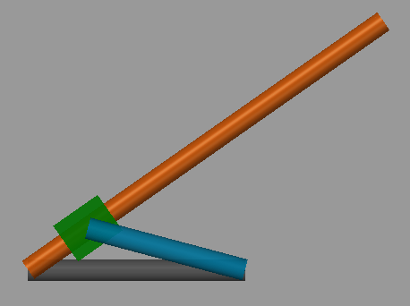
The following figure shows a mechanism which functions as an aiming system.

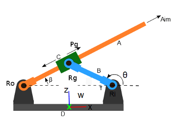
The problem is simplified to aiming within the plane of the mechanism. The figure shows the schematic sketch of the mechanism and only captures the essentials of how the mechanism operates (which is usually the case during the early stages of a design process). The link C can slide on the link A. A motor applies torque $\tau$ at the revolute joint Ri and the task is to track a particular trajectory of the revolute angle $\beta$.

Building the Mechanism

A key principle to follow is to begin with a simple approximation to get the basic mechanism working and then in subsequent iterations add complexity to the model. The recommended model building process can be broken down into the following steps:

The following sections describe these steps in more detail.

Identifying Rigid Bodies and Joints

The mechanism has four rigid bodies

The mechanism has the following joints

In addition, the rigid body D is rigidly connected to the world frame W since it is motionless.

Defining the Rigid Bodies and Their Interface

You define a rigid body by specifying its geometry, mass properties and interface with other parts. Each rigid body is identified and defined in isolation. In the above example, the mechanism is composed of four rigid bodies: A, B, C and D.

The rigid body A is shown in isolation below.

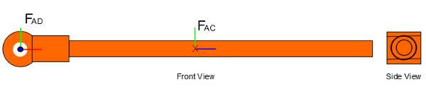
Once the shape of the object is defined and its density is specified, Simscape™ Multibody™ can compute the inertia automatically. Instead of defining the fairly complicated shape shown above, as a first approximation, you can define the shape of the rigid body as a simple cylinder.

The above shown rigid body can be defined in MATLAB using a high-level function like dcrankaim_approx_body_A which makes use of objects like simscape.multibody.RigiBody, simscape.mulitbody.Solid etc. This function takes input arguments like length, radius, density and color and returns a rigidbody object containing a cylindrical solid with one frame at the end of the link and the other at the center.

radius = simscape.Value(2,'cm');
length = simscape.Value(1,'m');
color = [0 0 1];
density = simscape.Value(2700,'kg/m^3') ;
bodyA = dcrankaim_approx_body_A(length,radius,density,color);

To understand the use of these different objects, let us take a look at the implementation of this function. In the dcrankaim_approx_body_A , we first import the packages needed to use Simscape Value, OperatingPoint and Simscape Multibody MATLAB classes.

import simscape.Value simscape.op.* simscape.multibody.*;

We then create an object of the class RigidBody. The RigidBody class is a container which can comprise of solids, inertias, graphics, frames (which act as interface to connect it to the other parts of Multibody system) and other rigid body objects.

link = RigidBody;

We then define and add a cylindrical solid to approximate the shape of BodyA. This is created using the cylindrical geometry, density, and its visual properties.

cylinder = Solid(Cylinder(radius, length),...
                 UniformDensity(density),...
                 SimpleVisualProperties(color));

addComponent(link,'Link', 'reference', cylinder);

Once we have defined the shape (first approximation) of the rigid body A and specified its density. We now has enough information to compute the inertial properties of the solid. You can define a simply shaped geometry in MATLAB using the following geometry classes.

These geometry objects are contained in the Solid class. Solids are characterized by geometry, inertia and visual properties and by using it with the above geometry objects, it allows us to create simple solids of different shapes. Solids are always rigid and always have an implicit reference frame, and the geometry and inertia are specified relative to this frame.

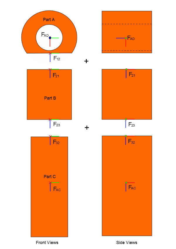
The interface of a rigid body is established by defining frames attached to the rigid body. A rigid body is connected to other parts of the mechanism via the rigidly attached frames. In Simscape Multibody, joints establish a time-varying relationship between two frames. For instance, the Revolute Joint establishes the relationship that the Z-axes of the attached frames are parallel and the origins of the frames are coincident. The Prismatic Joint establishes the relationship that the Z-axes of the attached frames are collinear and the X and Y axes are always parallel. Note that the frames themselves are defined independently of the joint; the joint only establishes a relationship between the already existing frames. Note also that the Z-axis is the axis of rotation in the case of the revolute joint and is the axis of sliding in the case of the prismatic joint. This information is essential when we define the interface of a rigid body by defining the frames rigidly attached to it.

In this example, the rigid body A has a cylindrical hole at one end that fits onto a peg so that A can rotate about the axis of the cylindrical hole. This suggests that a frame should be defined at the hole center with its Z-axis aligned with the axis of the hole (the axis of rotation). This frame is labelled as $F_{AD}$ above. The choice of orientation of the X and Y axes of $F_{AD}$ partly determines the zero configuration of the joint to which $F_{AD}$ would be connected (see discussion on Zero Configuration below). A also acts as the shaft on which part C slides. This suggests that a frame should be defined at the center of A (an arbitrarily selected position) with its Z-axis aligned along the length of A (along the direction of sliding). This frame is labelled as $F_{AC}$ above. The frames $F_{AD}$ and $F_{AC}$ define the interface for the rigid body A.

The following code shows how the frames are defined and added to the rigidbody A in the function dcrankaim_approx_body_A.

rt_Fad = RigidTransform( ...
         StandardAxisRotation(Value(90, 'deg'), Axis.PosY), ...
         StandardAxisTranslation(length/2, Axis.PosZ));

rt_Fac = RigidTransform( ...
         StandardAxisRotation(Value(180, 'deg'), Axis.PosY));

addFrame(link,'Fad', 'reference', rt_Fad);
addConnector(link,'Fad');

addFrame(link,'Fac', 'reference', rt_Fac);
addConnector(link,'Fac');

The frames $F_{AC}$ and $F_{AD}$ are defined with respect to the reference frame of the rigidbody.

To visualize this rigid body run the following code.

mb = Multibody;
addComponent(mb,'BodyA',bodyA);
cmb = compile(mb);
visualize(cmb,computeState(cmb,OperatingPoint),'BodyVizA');

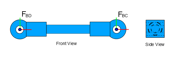
Now let us consider the rigid body B. The shape of the rigid body can again be approximated with a simple cylinder. The rigid body has cylindrical holes at both ends that fit onto pegs. The rigid body B can rotate about either hole axis. This suggests that two frames should be defined: one at each hole center with its Z-axis aligned with the axis of the hole.

The function dcrankaim_approx_body_B shows how the RigidBody, Solid and RigidTransform objects have been used to define the shape, inertia and interface of the rigid body B.

radius = simscape.Value(2,'cm');
length = simscape.Value(1,'m');
color = [0 0 1];
density = simscape.Value(2700,'kg/m^3') ;

bodyB = dcrankaim_approx_body_B(length,radius,density,color);

To visualize this rigid body run the following code.

mb = Multibody;
addComponent(mb,'BodyB',bodyB);
cmb = compile(mb);
visualize(cmb, computeState(cmb,OperatingPoint),'BodyVizB');

A similar approach can be taken for building a first approximation of the rigid body D.

Now let us consider the rigid body C.

This rigid body has a cylindrical hole that slides on a peg. It also has a peg about which another body can rotate. This suggests the need to define two frames: one at the center of the hole with its Z-axis along the axis of the hole, and the other at the center of the peg with its Z-axis along the axis of the peg. These are marked as $F_{CA}$ and $F_{CB}$ above.

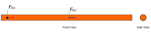
The shape of the rigid body C can be approximated with a simple cuboid. In the first approximation of the rigid body, the offset between the origins of frames $F_{CB}$ and $F_{CA}$ can also be made zero. This results in the simplified representation of rigid body as shown below.

The function dcrankaim_approx_body_C shows how the RigidBody, Solid and RigidTransform objetcs have been used to define the shape, inertia and interface of the rigid body C.

brickdim =  simscape.Value([10, 8, 8], 'cm');
density = simscape.Value(2700,'kg/m^3') ;
color = [0 0 1];
bodyC = dcrankaim_approx_body_C(brickdim,density,color);

Assembling the Individual Bodies Using Joints

All the individual bodies were built in isolation. The process of assembly involves establishing relationships (using joints) between the frames attached to the rigid bodies. The following joints establish all of the necessary relationships between the frames to assemble the mechanism.

The function dcrank_aiming_mechanism_v1 shows how objects like Mulitbody and Joints are used to assemble individual rigid bodies. The function takes the length of each of the cylindrical links BodyA, BodyC, BodyD and the dimensions of the slider link BodyB as the input arguments and returns the multibody object as the output.

bodyA_l = Value(80,'cm'); 
bodyB_l = Value(30, 'cm');
bodyC_dim = Value([10, 8, 8], 'cm');
bodyD_l = Value(40, 'cm'); 
dcrankAimMech_mb = dcrank_aiming_mechanism_v1(bodyA_l,bodyB_l,bodyC_dim,bodyD_l);

To understand how this function assembles the mechanism, let us look at some its implementation.

In dcrank_aiming_mechanism_v1, we first create a Multibody object, which acts as container for variety of other components like RigidBodies , Solids, Joints , RigidTransforms.

dcrankAimMech_mb = Multibody;

We then add the World frame to the Multibody by using its addComponent method.

addComponent(dcrankAimMech_mb,'World', WorldFrame());

Then BodyA , BodyB , BodyC and BodyD are created using the RigidBody object, as discussed in the above sections.

% add body_a
bodyA_l = Value(80,'cm'); 
bodyA_r = simscape.Value(2,'cm');
bodyA_color = [1 0.6 0];
bodyA_density = simscape.Value(2700,'kg/m^3') ;
body_a = dcrankaim_approx_body_A(bodyA_l,bodyA_r,bodyA_density,bodyA_color);

% add body_b
bodyB_l =  Value(30, 'cm');
bodyB_r = simscape.Value(2,'cm');
bodyB_color = [0 0 1];
bodyB_density = simscape.Value(2700,'kg/m^3') ;
body_b = dcrankaim_approx_body_B(bodyB_l,bodyB_r,bodyB_density,bodyB_color);

% add body_c
bodyC_dim = Value([10, 8, 8], 'cm');
bodyC_color = [0 1 0];
bodyC_density = simscape.Value(2700,'kg/m^3') ;
body_c = dcrankaim_approx_body_C(bodyC_dim,bodyC_density,bodyC_color);

% add body_d
bodyD_l = Value(40, 'cm'); 
bodyD_r = simscape.Value(2,'cm');
bodyD_color = [0.2 0.2 0.2];
bodyD_density = simscape.Value(2700,'kg/m^3') ;
body_d = dcrankaim_approx_body_D(bodyD_l,bodyD_r,bodyD_density,bodyD_color);

Once all the 4 bodies are created, we add them to the Multibody container object using its addComponent method.

addComponent(dcrankAimMech_mb,'body_a', body_a);
addComponent(dcrankAimMech_mb,'body_b', body_b);
addComponent(dcrankAimMech_mb,'body_c', body_c);
addComponent(dcrankAimMech_mb,'body_d', body_d);

The mechanism has 4 joints - 3 revolutes and 1 prismatic. We create and add them using the RevoluteJoint and PrismaticJoint objects.

rJoint = RevoluteJoint;
pJoint = PrismaticJoint;

addComponent(dcrankAimMech_mb,'Ro', rJoint);
addComponent(dcrankAimMech_mb,'Ri', rJoint);
addComponent(dcrankAimMech_mb,'Rg', rJoint);
addComponent(dcrankAimMech_mb,'P', pJoint);

Now, we have all the required components for the mechanism. However, we still need to connect these components. We add these connections using the connect and connectVia methods of the Multibody object by connecting the appropriate RigidBody frames to the Base and Follower frames of the appropriate Joints.

connect(dcrankAimMech_mb,'World/W', 'body_d/Fdw');
connectVia(dcrankAimMech_mb,'Ro', 'body_d/Fda', 'body_a/Fad');
connectVia(dcrankAimMech_mb,'P',  'body_a/Fac', 'body_c/Fca');
connectVia(dcrankAimMech_mb,'Rg', 'body_b/Fbc', 'body_c/Fcb');
connectVia(dcrankAimMech_mb,'Ri', 'body_d/Fdb', 'body_b/Fbd');

The effort that went into carefully defining the interfaces of all of the rigid bodies (i.e. the frames attached to them) made it very easy to complete the mechanism by simply adding and connecting the joints between the appropriate frames. However, at this point the resulting assembly may or may not be in the desired configuration since the mechanism can be assembled into multiple configurations. The function dcrankaim_assembly_failure shows the assembled mechanism.

dcrankAimMech_mb = dcrankaim_assembly_failure(bodyA_l,bodyB_l,bodyC_dim,bodyD_l);

Using computeState Method to Identify Problems

In the function above, an intentional mistake has been made in the definition of the frame $F_{CA}$ attached to rigid body C. This causes the assembly to fail. The figure below shows the desired and actual orientations of the frame $F_{CA}$.

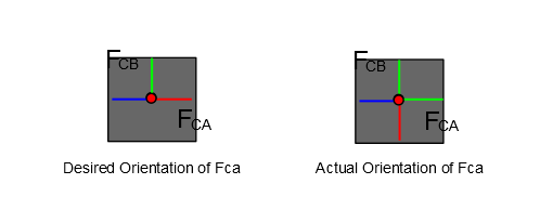
The orientation of $F_{CA}$ has to be corrected by a rotation of 90 deg about the Z-axis. To identify this issue, we first compile the multibody using the compile method of the Multibody object.

compiled_mb = compile(dcrankAimMech_mb);

Then we use the computeState method of the compiled multibody object for a default OperatingPoint.

state = computeState(compiled_mb,simscape.op.OperatingPoint)

state = 
  State:

  Status: PositionViolation

  Assembly diagnostics:
  x
    Ro
        Joint successfully assembled
        Rz
            Free position value: +0.000377073 (deg)
            Free velocity value: +0 (deg/s)
    P
        Joint successfully assembled
        Pz
            Free position value: +0.3 (m)
            Free velocity value: +0 (m/s)
    Ri
        Joint successfully assembled
        Rz
            Free position value: +0.00087955 (deg)
            Free velocity value: +0 (deg/s)
    Rg
        Joint not assembled due to a position violation.
        Rz
            Free position value: N/A (deg)
            Free velocity value: N/A (deg/s)

The State object returned by the computeState method indicates if the attempt to compute a state was successful or not. In this case, it reported indicating that there is a PositionViolation and that the joint Rg is not assmebled due to a position violation. In this example it is in fact true that an error was made in the specification of the frame $F_{CA}$ which would cause a position violation.

Changing the parameters of the rigid transform ax_fca.BaseAxis2, from Axis.NegZ to Axis.PosZ in dcrankaim_approx_body_C_assembly_failure fixes the problem and allows the assembly to succeed.

Zero Configuration of Joints

The Zero Configuration of a joint is defined as the relative position and orientation between the base and follower frames when all of the joint angles are zero. For almost all of the joints in Simscape Multibody, the base and follower frames are identical in the zero configuration: their origins are coincident, and their axes are aligned. One defines the relative position and orientation between two bodies connected by a joint when the joint angles are zero by adjusting the positions and orientations of the base and follower frames on their respective bodies.

Consider, for example, the rigid bodies B and C and the joint Rg connecting them. The frames $F_{CB}$ and $F_{BC}$ are the base and follower frames of the joint Rg. The figure below shows how different choices of orientations for the frame $F_{CB}$ attached to rigid body C result in different assembled configurations when the joint angle is zero. The choice of orientation of the frames must be made with the desired zero configuration in mind.

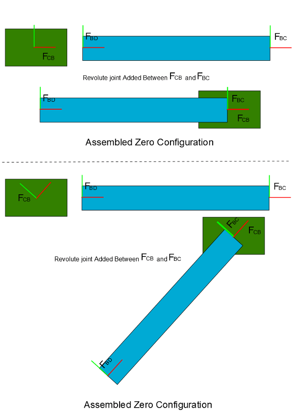
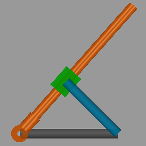
In the aiming mechanism, the choice of frame orientations leads to a default assembled configuration in which the central axes of all of the bodies lie along the same line.

Guiding Assembly Using Operating Points

Visualize the mechanism created using dcrank_aiming_mechanism_v1 (contains the fix for the errors found in dcrankaim_approx_body_C_assembly_failure ) using the following code.

dcrankAimMech_mb = dcrank_aiming_mechanism_v1(bodyA_l,bodyB_l,bodyC_dim,bodyD_l);
cmb = compile(dcrankAimMech_mb);
visualize(cmb,computeState(cmb,simscape.op.OperatingPoint),'vizAssembly');

It can be seen that all of the bodies are collapsed onto a common line; this is the default assembly configuration. In this configuration, all of the revolute joint angles are zero. Thus, the base and follower frames of each revolute joint are coincident and aligned with each other; the corresponding frame pairs are: $F_{DA}$ and $F_{AD}$, $F_{CB}$ and $F_{BC}$ and $F_{BD}$ and $F_{DB}$. In contrast, the frame $F_{CA}$ is translated from frame $F_{AC}$, thus the joint Pg is not in its zero state. We can view the computeState result to view the values of the joint positions in this assembled configuration. This is currently not a desirable assembly configuration.

The configuration depicted in the schematic diagram of the mechanism is the desired initial assembly configuration. From the schematic diagram we can see that in the initial configuration the angle $\beta$ is about 35 deg. The assembly algorithm can be guided by specifying joint position and velocity targets using the OperatingPoint. In this example, the position target for the joint Ro can be set to guide assembly into the desired initial configuration using operating points. The target priority has been set as High. Since this is the only target for the system that computeState is able to achieve exactly.

op = simscape.op.OperatingPoint;
op('Ro/Rz/q') = simscape.op.Target(35, 'deg', 'high') ;
% Note: As an aid to obtain the joint primitive paths needed by the operating point (i.e
% 'Ro/Rz/q'), use jointPrimitivePaths method of the Multibody object.
% For example, in this case we can view all the joint primitive paths using
% >> dcrankAimMech_mb.jointPrimitivePaths;

Now compute the state for the above operating point and check the State object to see that the joint target for Ro has been met exactly.

compiled_mb = dcrankAimMech_mb.compile();
state = compiled_mb.computeState(op)

state = 
  State:

  Status: Valid

  Assembly diagnostics:
  x
    Ro
        Joint successfully assembled
        Rz
            High priority position target +35 (deg) achieved
            Free velocity value: +0 (deg/s)
    P
        Joint successfully assembled
        Pz
            Free position value: +0.120952 (m)
            Free velocity value: +0 (m/s)
    Ri
        Joint successfully assembled
        Rz
            Free position value: +84.8864 (deg)
            Free velocity value: +0 (deg/s)
    Rg
        Joint successfully assembled
        Rz
            Free position value: -49.8864 (deg)
            Free velocity value: +0 (deg/s)

Visualize it to view the new configuration.

compiled_mb.visualize(state,'vizAimMech');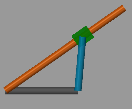

Unfortunately, the assembled configuration is not the intended one because the rigid body B is not aligned as indicated in the schematic diagram. Attempting to specify the joint angles of both $$Ro$$ and $$Ri$$ exactly is an over-specification for this one degree-of-freedom mechanism. This is not prohibited, but if there is a conflict, neither target may be met. Moreover, the desired angle of joint Ri is not even known exactly.

In this situation, a convenient approach is to leave the high-priority target of 35 deg on Ro but to specify the angle of Ri through a low-priority position target. The latter provides an approximate value, or hint, for the desired joint angle. In this case, it is obvious that the angle $\theta$ should be obtuse; 150 deg is a rough estimate of its desired value. This target is set for joint Ri with a priority of Low.

op('Ri/Rz/q') = simscape.op.Target(150, 'deg', 'low') ;
compiled_mb = compile(dcrankAimMech_mb); 
state = computeState(compiled_mb,op);
visualize(compiled_mb,state,'vizAimMech');

The assembled configuration after setting the new target is shown below.

To simulate the mechanism, we can create a simulink model by using the makeBlockDiagram method of the Multibody object.

makeBlockDiagram(dcrankAimMech_mb,op,'dcrankAimMech_model');

Once the model is created, simulate the model (Ctrl-T) to view the motion of the mechanism under gravity.

Adding Detail to the Rigid Bodies

Now that the basic model is working, the next step is to add detail to make the model more realistic and accurate. Perhaps the first version of the model was created when detailed information about the geometry of the rigid bodies was not yet available. Having carefully established the interfaces of the rigid bodies, it is fairly easy to add detail to each of the rigid bodies without affecting/changing the rest of the model.

As an example, consider adding detail to the rigid body A while keeping its interface unchanged. The figure below shows rigid body A as a composition of simpler bodies. The interface exposed by rigid body A is still the pair of frames $F_{AD}$ and $F_{AC}$. Their positions and orientations remain unchanged. The frames $F_{12}$ , $F_{21}$ , $F_{23}$ and $F_{32}$ are internal to the rigid body and should be created to assemble the individual pieces of the rigid body into a whole. The function dcrankaim_detailed_body_A shows the construction of the complex version of the rigid body A.

The second version function dcrank_aiming_mechanism_v2 was obtained from dcrank_aiming_mechanism_v1 by just replacing the call to the function dcrankaim_approx_body_A to dcrankaim_detailed_body_A to create complex version of rigid body A. Because the interface remained constant, it was a simple operation. Create and view the updated mechanism using the following code.

dcrankAimMech_mb = dcrank_aiming_mechanism_v2(simscape.Value(80,'cm'),simscape.Value(30,'cm'),simscape.Value([8 8 8],'cm'),simscape.Value(40,'cm'));
cmb = compile(dcrankAimMech_mb);
op = OperatingPoint;
op('Ro/Rz/q') = Target(35, 'deg', 'high') ;
op('Ri/Rz/q') = Target(150, 'deg', 'low') ;
visualize(cmb,computeState(cmb,op),'vizMechDetailed');

Similarly, details can be added to the other rigid bodies by following the above discussed process.

Summary

In summary, we took the following steps to build a multibody system in MATLAB: