Compounding Body Elements

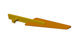
It is often simpler to specify the attributes of several simple solids than those of a single complex body. Compounding is a modeling strategy whereby you can model a body as a combination of simpler body elements. You can use compounding to obtain complex geometries and inertias that you cannot otherwise (or easily) specify. The RightWing body in the PointOnCurveExample model, for example, is a product of this modeling strategy.

An Example of a Compound Body

Create a Compound Geometry

Combine three general Extruded Solid shapes using Rigid Transform blocks to specify the fixed spatial relationships shared by the solid reference frames. The result of this example is not merely a compound solid geometry—it is a compound body. You must use the deliberately incomplete model DocCompoundLinkExample that by default comes with your Simscape™ Multibody™ installation.

Explore the Compound Body Model

Start by exploring the DocCompoundLinkExample model and the geometry variables defined in its workspace:

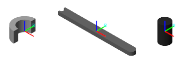
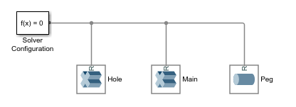
At the MATLAB^® command prompt, enter openExample("sm/DocCompoundLinkExample"). The model opens. In it are six unconnected blocks—three solid blocks, two Rigid Transform, and one Solver Configuration.
The solid blocks represent the elementary sections of a binary link and the Rigid Transform blocks the spatial relationships between the solid reference frames. The Solver Configuration block is required only for visualization in Mechanics Explorer.
In the Modeling tab, click Model Explorer. Model Explorer is a Simulink^® tool that you can use to explore your model workspace. All the relevant solid dimensions, including the general Extruded Solid cross-sections, are defined there.
In the Model Hierarchy pane, located on the left, expand the node named after your model and select the Model Workspace subnode. The Model Workspace pane opens on the right prefilled with several lines of MATLAB code.
```
% Body Geometry Parameters
l = 20;     % Hole-to-hole distance
w = 2;      % Link width
d = 1.2;    % Hole diameter
t = 1;      % Link thickness

% Main Solid Cross-section:
A = linspace(-pi/2,pi/2)';
B = linspace(pi/2,-pi/2)';
csRight = [l/2+w/2*cos(A) w/2*sin(A)];
csLeft = [-l/2 w/2; -l/2 + d/2*cos(B) d/2*sin(B); -l/2 -w/2];
csMain = [csRight; csLeft];

% Hole Solid Cross-section:
C = linspace(pi/2,3*pi/2)';
D = linspace(3*pi/2,pi/2)';
csHole = [w/2*cos(C) w/2*sin(C);
d/2*cos(D) d/2*sin(D)];
```
This code defines the [x, y] coordinates of the General Extruded Solid cross-sections. The cross-sections are parameterized in terms of the relevant solid dimensions, namely length, width, and hole diameter. Note the link dimensions specified in the code. The distance between the link holes (variable l), is 20 in what will later be units of cm. The link width (w) is 2 and the hole diameter (d) 1.2 in the same units.
Open each solid block dialog box. The visualization pane shows the solid geometry, derived partly from the code in the model workspace, corresponding to the respective block. Two of the solids are general Extruded Solid blocks, and one is a Cylindrical Solid block.
On the toolstrip of the visualization pane, click the Toggle visibility of frames button. The visualization pane displays the solid reference frame. The placement of a reference frame relative to a solid geometry becomes important when considering the rigid transforms that you must apply between the various solid reference frames.

Combine the Solids Through Rigid Transforms

Complete the model by rigidly connecting the solids and specifying their spatial relationships:

Connect the solid blocks as shown in the figure. The solid reference frames are, for the moment only, coincident with each other.
Drop the Rigid Transform blocks on the connection lines as shown in the figure. Simulink automatically connects the frame ports to the connection lines.
Pay special attention to the port positions—the B ports should both face the Extruded Solid block named Main. Flipping the port connections would change the relative placement of the solids in the final body.
In the dialog box of the Rigid Transform block named Main-to-Hole Transform, specify the Translation parameters listed below. These parameters describe a translation of half the binary link length along the -x axis of the base (B) frame—in this model held coincident with the reference (B) frame of the solid named Main.
- Method: Standard Axis
- Axis: -X
- Offset: l/2, units of cm
In the dialog box of the Rigid Transform block named Main-to-Peg Transform, specify the Translation parameters listed below. These parameters describe a translation of half the binary link length along the +x-axis and a translation equal to the binary link thickness along the +z-axis of the base (B) frame.
- Method: Cartesian
- Offset: [l/2 0 t], units of m
In the Modeling tab, select Update Model. Mechanics Explorer opens with a visualization of the binary link model. The body is compound—it comprises multiple solids—and can therefore be visualized in its entirety using Mechanics Explorer only. For emphasis, the solids are shown in different shades of gray.

A More Detailed Cross-Section Example

For an example showing how to specify a General Extruded Solid cross-section, see Try It: Define a Simple Cross-Section. The cross-section in that example is based on a similar, though not identical, model of a binary link. That link is treated as a simple body—one modeled as a single solid—with neither pegs nor holes. However, the strategy demonstrated there applies to other General Extruded Solid cross-sections as well. For an extension of that example showing how to include holes in a cross-section, see Try It: Define a Cross-Section with Two Holes.

Create a Compound Inertia

While it is more commonly used to represent complex geometries, compounding serves also to represent complex inertias. In particular, you can combine the inertia of a positive mass with the inertia of a negative mass, effectively subtracting one from the other.

Use this strategy to subtract the inertia associated with a bore from a cylindrical solid originally modeled without one. Represent the dense and hollow regions using Cylindrical Solid blocks. Set the cylinder length to 1 m and the radius to 0.25 m:

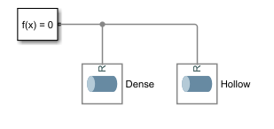
At the MATLAB command prompt, enter smnew. A new model based on the Simscape Multibody template opens up. The model contains commonly used blocks and is configured with suitable solver settings for multibody models.
Add two of the Cylindrical Solid blocks and connect them to the Solver Configuration blocks. The frame connection line between the blocks make their reference frames coincident in space. You can delete the remaining blocks.
In the dialog box of the leftmost Cylindrical Solid block, set the Radius parameter to 0.25 m, and the Length parameter to 1 m. Name this block Dense.
In the dialog box of the rightmost Cylindrical Solid block, set the Radius parameter to 0.20 m, and the Length parameter to 1 m. Name this block Hollow.
Set the Inertia > Density parameter of the Hollow block to the negative of the value used in the Dense block: -1000 kg/m^3. The compound body represented by the Cylindrical Solid blocks now has the inertia of a hollow cylinder with a bore 0.2 m in radius.
Expand the Inertia > Derived Values node and click the Update button to display the inertia parameters of the Hollow solid. Do the same for the Dense solid. The mass and moments of inertia have opposite signs, as expected from the density inputs.