Modeling Extrusions and Revolutions
Extrusions and Revolutions
For solids with custom cross-sections, the Extruded Solid and Revolved Solid blocks enable you to create truer solid representations than simpler shapes such as Brick Solid, Cylindrical Solid, and Spherical Solid often allow. Use them when modeling solids that have arbitrary yet constant cross-sections along or about an axis. The Extruded Solid block can either be a General extrusion or a Regular extrusion.
What is the Extruded Solid Block?
A general extrusion is a linear sweep of a custom cross-section along an axis that is normal to the cross-section plane. The sweep spans the length specified in the Extruded Solid block dialog box. The cross-section can have an arbitrary outline and one or more hollow sections—though the rules for specifying cross-sections differ slightly when holes are present.
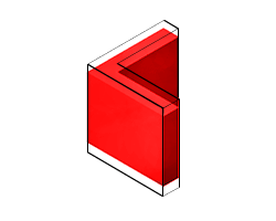
General extrusion examples include straight beams, plates, spars, struts, and rods. The figure shows an angle beam, a general extrusion whose cross-section consists of two thin rectangles arranged in an L shape. The Extruded Solid block sweeps the L shape linearly out of the cross-section plane to obtain the final beam geometry.
General Extruded Solid Block as a Linear Sweep

A Note on Extruded Solid Shapes. The Extruded Solid block provides a second extrusion shape, named Regular extrusion. This shape is a simpler version of General extrusion and is suited only for solids whose cross-sections are regular polygons—those with sides of the same length. The cross-section outline is fixed by the number of sides of the polygon and it cannot contain holes.
What is the Revolution Solid block?
Use the Revolved Solid block to make an angular sweep of a cross-section about an axis that lies on the same plane as the cross-section. The sweep can span a full revolution or a lesser angle between 0 and 360 degrees. As with extruded shapes, the cross-section can have an arbitrary outline with or without holes.
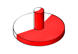
Revolved examples include cones, domes, pistons, gear shafts, and pipe bends. The figure shows a cylindrical peg, a Revolved Solid whose cross-section, like the angle beam, consists of two thin rectangles arranged in an L shape. The Revolved Solid block sweeps the L shape about an axis lying on the cross-section plane to obtain the final peg geometry.
Revolved Solid as an Angular Sweep

The Cross-Section Profiles
You specify the cross-sections numerically, as MATLAB® matrices populated with the coordinate pairs of select cross-section points. Each matrix row provides a coordinate pair for one point. There is no upper bound on the number of rows of a coordinate matrix, but a minimum of three is required to completely define a closed shape.
% Coordinate Matrix Example:
% Square Cross-Section with Center at [0, 0] and Side Length 2
[
-1 -1; % Lower left corner
1 -1; % Lower right corner
1 1; % Upper right corner
-1 1; % Upper left corner
]
The coordinate pairs are treated as (x, y) values in the case of extruded shapes and as (x, z) values—specified in that order—in the case of revolved shapes. The coordinates are resolved in the reference frame of the Extruded Solid or Revolved Solid block, with the (0, 0) pair coinciding with the origin of that frame. It is common practice to parameterized the coordinates in terms of MATLAB variables associated with key solid dimensions—for example, radius or length.
From Coordinates to Cross-Sections
The coordinate pairs connect sequentially in the order implicit in the coordinate matrix. The connections are by means of straight line segments. The result is a closed polyline that separates the region to be filled with material (the solid part) from the region to be left hollow (any holes that might be present and the empty surroundings).
The boundary between the two regions is such that, as you proceed along the polyline from one point to the next, the solid region lies to your left and the hollow region to your right. The first and last coordinate pairs are often the same, but if they are not, a connection line is inserted between them to ensure that the cross-section is in fact closed. The animated figure shows the drawing of a binary link cross-section without holes.

Note that the cross-section is invalid if at any point the polyline crosses itself. However, it is okay for two line segments to be arbitrarily close or even coincident with each other. In fact, you can exploit this property to specify a cross-section that has one or more holes.
A Special Constraint for Revolutions
Revolved Solid coordinate matrices are subject to a special constraint: x-coordinates cannot be negative. This rule follows partly from the revolution axis (z) used by the Revolved Solid block. When sweeping the cross-section, any areas to the left of this axis (those with negative x-coordinates) become overlapped with those to the right (positive x), resulting in an unexpected solid geometry. To prevent this issue, an error is issued if a Revolved Solid cross-section is found with negative x-coordinates.
Try It: Define a Simple Cross-Section
Consider the cross-section shown in the figure. This cross-section belongs to a binary link with round ends and no holes. Parameterize the cross-section in terms of the dimensions shown and specify it in the form of a coordinate matrix.
Binary Link Cross-Section (No Holes)

Start by opening a new MATLAB script and save it in a convenient location under the name
modelParams. Add two variables for the dimensions
shown in the figure, length (l) and width
(w). Set the length to 20 and the
width to 2 (in what will later be units of
cm).
l = 20;
w = 2;
Define the round ends as semicircles. First, generate two arrays with the angular spans of the left and right ends. These arrays enable you to parameterize the (x, y) coordinates using simple trigonometric expressions. Each array has five points, but for smoother shapes you can specify more. The transpose symbol (') ensures that A and B are column arrays.
A = linspace(-pi/2, pi/2, 5)';
B = linspace(pi/2, 3*pi/2, 5)';
Define the coordinate matrices of the right end (csRight) and left end (csLeft). The first column of each matrix corresponds to the x-coordinate. The second column corresponds to the y-coordinate. The x-coordinates of the two ends are offset in opposite directions by l/2.
csRight = [l/2 + w/2*cos(A) w/2*sin(A)];
csLeft = [-l/2 + w/2*cos(B) w/2*sin(B)];
Combine the coordinate matrices into a single matrix named cs. This is the matrix that you must specify in the Cross-Section parameter of the Revolved Solid block. Note that the straight segments of the cross-section are automatically generated when the end points of the semicircles are connected.
cs = [csRight; csLeft];You can visualize the cross-section outline using the MATLAB plot command. Enter the code shown below at the MATLAB command prompt.
figure; hold on; axis equal;
plot(cs(:,1), cs(:,2), 'Color', [0.6 0.6 0.6], 'Marker', '.',...
'MarkerSize', 9, 'MarkerEdgeColor', [1 0 0]);
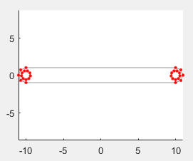
The plot shows the cross-section of the binary link. The points in the coordinate matrix are shown as red dots. The resulting cross-section outline is shown as a light gray line. Notice that the end sections each comprise five points—the number specified in the angular span arrays.

Cross-Sections with Holes
The coordinate matrix should always represent a single continuous path. This rule works well when specifying a cross-section without holes but it demands extra care when holes exist. Because the outline of a hole is not contiguous with the outline of the cross-section, you must now add a thin cut between the two. The cut enables you to traverse the cross-section and hole outlines in a single loop.
Consider a binary link with a hole at one end. The cross-section of this body comprises two closed paths—one for the cross-section outline, the other for the hole. The paths are physically separated. However, you can connect them by cutting each path at a vertex and joining the cut vertices with additional line segments. The animated figure shows the drawing of a binary link cross-section with one hole.

You can extend this approach to cross-sections with multiple holes. Note that each hole must have a cut. There is no single best way to approach the cuts. The key is to plan them so that you can traverse the cross-section—and all of its holes—in a single continuous path while keeping the polyline from intersecting itself. The animated figure shows the drawing of a binary link cross-section with two holes.

Try It: Define a Cross-Section with Two Holes
Modify the coordinate matrix in your modelParams script to include two identical holes as shown in the figure. Save the script often as you go.
Binary Link Cross-Section (Two Holes)

Start by adding a new variable for the hole diameter (d). Set the diameter to 1.2 (in what will later be units of cm).
d = 1.2;Generate a new angular span array for the left and right holes. The holes are drawn in the same order and a single array suffices. The array elements are ordered in a clockwise direction, ensuring that when generating the cross-section the solid region stays to the left. The number of array elements has doubled to reflect the wider angular span of the holes (360° vs 180°).
C = linspace(3*pi/2, -pi/2, 10)';Define the outlines of the left hole (csLeftHole), the right hole (csRightHole), and the connection line between the two (csConnLine). The x-coordinates are shifted left by half the length (l/2) for the left hole and right by the same distance for the right hole.
csLeftHole = [-l/2 + d/2*cos(C) d/2*sin(C)];
csRightHole = [+l/2 + d/2*cos(C) d/2*sin(C)];
csConnLine = [-l/2 -w/2; +l/2 -w/2];
Add the new coordinate matrices to the existing cs matrix. The order of the matrices determines the order in which the complete cross-section is drawn. The result is a variable that you can specify in the Cross-section parameter of the Revolved Solid block.
cs = [csRight; csLeft; csLeftHole; ...
    csConnLine; csRightHole];
As before, you can visualize the cross-section outline using the MATLAB plot command. Ensure that the plotting code shown below is included in your script. Then, run the script to generate the plot.
figure; hold on; axis equal;
plot(cs(:,1), cs(:,2), 'Color', [0.6 0.6 0.6], 'Marker', '.',...
'MarkerSize', 9, 'MarkerEdgeColor', [1 0 0]);
The plot shows the cross-section of the binary link. The points in the coordinate matrix are shown as red dots. The resulting cross-section outline is shown as a light gray line. Note that the hole sections each comprise ten points—the number specified in the angular span arrays.

From Cross-Sections to Solids
The z-axis of the reference frame serves as the sweep axis in both the Extruded Solid and Revolved Solid blocks. The specified cross-section is swept along this axis in the case of Extruded Solid block and about this axis in the case of the Revolved Solid block. The sweep is symmetrical with respect to the cross-section plane: it runs half of the sweep length or angle in each direction of the sweep axis. This symmetry leaves the cross-section plane—and therefore the origin of the reference frame—halfway between the ends of the sweep.
Try It: Use Your Cross-Section to Model a Solid
Open a new Simulink® model and, from the Bodies library, add a Extruded Solid block. You can click the model canvas, type the block name, and make a selection from the options shown. Save the model in a convenient location as
binaryLinkSolid.In the Extruded Solid block dialog box, set the Geometry parameters as shown in the table. Set the parameter units to
cm. The Cross-Section parameter is defined in terms of thecsvariable in yourmodelParamsscript.Parameter Value Cross-Section csLength 1 Load your
modelParamsscript to your model workspace:In the Modeling tab, click Model Explorer. You use this tool to load the
modelParamsscript that you previously created onto your model workspace.In the Model Hierarchy pane, expand the node corresponding to your model (binaryLinkSolid) and select Model Workspace.
In the Model Workspace pane, set the Data source parameter to
MATLAB Fileand browse for yourmodelParamsscript. Click the Reinitialize from Source button to load variables defined in the script.
In the Extruded Solid block dialog box, click the Update Visualization button,
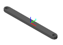
 . The visualization pane refreshes with the final solid geometry.
 Click the Fit to View button to scale the binary link to the size of the visualization pane. Click the Toggle visibility of frames button to show the solid reference frame. The reference frame origin coincides with the [0, 0] cross-section coordinate and lies halfway between the extrusion ends.

Note the jagged appearance of the round ends and holes. This effect results from the small number of points used in the round portions of the coordinate matrix—
csLeftEnd,csRightEnd,csLeftHole, andcsRightHole. Increase the number of elements in the angular span arrays to obtain a smoother geometry.