Tolerance Study Using Monte Carlo Simulations in Resonant LLC DC-DC Converter
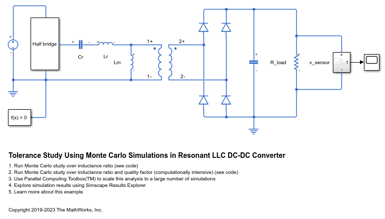
This example shows how to use Simscape™ Electrical™ to perform a Monte Carlo analysis to optimize the design of an LLC resonant DC-DC converter when some of its components have tolerances.
Motivation
When designing an electrical system, some components might possess certain tolerance on some key parameters (for example the inductance of an inductor). Looser tolerance components usually have a lower cost, so it is cost-effective to choose them.
However, component tolerance impacts system performance, introducing a variability on some key specifications. This example shows you how to choose design options that minimize the variability of the entire system.
In this example, an LLC resonant DC-DC converter comprises capacitors and inductors with a given tolerance, and there are several choices for design parameters that provide the desired gain output. The goal is to find which of these design choices have the minimum output gain tolerance, or global system variability.
Monte Carlo Method
The components' statistical variability influences the global system statistical variability. Monte Carlo method consists of inferring an estimation of this influence by statistical repetition. A given known distribution generates the component parameter values and then a simulation is performed to obtain system level results. Simulations are repeated many times. If the number of simulations is large enough, the system output distribution is reasonably well inferred.
Model

In this particular design, the control system has been chosen to be very simple: a fixed switching frequency in open-loop.
Theoretical Approximation for Output Voltage Gain
For this converter, a first harmonic approximation to compute output voltage gain from design parameters is:

in which  and
and  are the inductance ratio and quality factor, which directly depend on the inductances and capacitance of the components of interest in this study.
We will use this formula to compute an approximation to the expected output gain when components are perfect (do not have any tolerance).
Specifying Component Tolerance
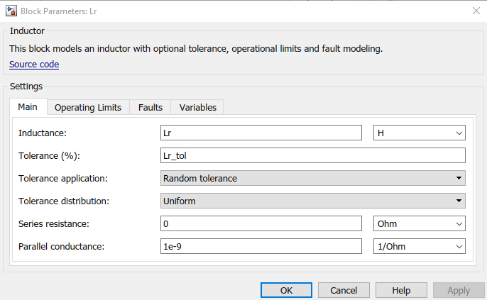
You can specify the component tolerances in the block mask. For example, in the inductor, you can apply a tolerance value with a uniform distribution on a certain range of inductances.

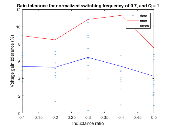
System Tolerance Study (Over Ln Only)
After you apply the tolerances (20% for the inductors and 7% for the capacitor in this example), you run multiple simulations during which the indunctances and capacitance are randomly generated at t=0 with a uniform distribution. The output gain measured on the load varies each time, as the system is different during each simulation due to the tolerances. For a fixed design choice (fixed  and fixed
  ), multiple repeated Monte Carlo simulations infer a statistical distribution of the output voltage.
In this section, to find out which configuration gives a lower output voltage gain variability, you fix a value of  and change the value of
  over a range you want to study.
This script will run 50 simulations.

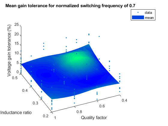
System Tolerance Study (Over Ln and Quality Factor)
To study the system tolerance over  and the quality factor, change the value of
  as well. A grid of values for L_N and Q is then selected and, for every configuration, the model estimates the output gain distribution through repetition.
This script will run 160 simulations.


Advantages of Parallel Computing
Simulating hundreds or thousands of times is computationally expensive and time consuming. To reduce computation time, you can run multiple simulations in parallel. This is especially advantageous for independent Monte Carlo simulations.
For this workflow, Parallel Computing Toolbox™ is used to speed up the process and scale it up to a higher number of simulations.
Up until this point, this example worked on a grid of 4x4 configurations with 10 simulations each. This figure shows an animation of the same workflow scaled up to a grid of 17x17 configurations with 100 simulations each.

The surface plot shows the worst case scenario with the maximum tolerance found for each configuration. The surface plot shapes to a more reliable representation of the distribution of the output gain tolerances as the number of simulation increases. The configuration with  and
and  has the lowest possible output gain tolerance equal to around 9%.
To reproduce these results, use the MonteCarloResonantLLCDCDCParallel script. This script uses functions and methods from the Parallel Computing Toolbox™ such as parsim, batchsim, parcluster, Simulink.SimulationInput.setModelParameter, Simulink.SimulationInput.setVariable, and other useful tools.
See Also
Simscape Blocks
Functions
parsim|parpool(Parallel Computing Toolbox) |parcluster(Parallel Computing Toolbox)