Tune an Electric Drive

This example shows how to tune an electric drive using a cascade control structure.

Cascade Control Structure

The figure shows a feedback control loop that uses a cascade control structure. The outer speed-control loop is slower acting than the inner current-control loop.

Equations for PI Tuning Using the Pole Placement Method

To satisfy the required control performance for a simple discrete plant model, G_f(z^-1), use a closed loop PI control system G_PI(z^-1). The transient performance can be expressed in terms of the overshoot. The overshoot decreases relative to the damping factor:

$σ = e^{\frac{- π ξ}{\sqrt{1 - ξ^{2}}}}$

where,

σ is overshoot.
ξ is the damping factor.

The response time, t_r, depends on the damping and the natural frequency, ω_n, such that:

If ξ < 0.7,
$t_{r} ≅ \frac{4}{ω_{n} ξ} .$
If ξ ≥ 0.7,
$t_{r} ≅ \frac{6 ξ}{ω_{n}} .$

The general workflow for designing a PI controller for a first-order system is:

Discretize the plant model using the zero-order hold (ZOH) discretization method. That is, given that the first-order equation representing the plant is

$G (s) = \frac{K_{m}}{T_{m} s + 1},$
where,
- K_m is the first-order gain.
- T_m is time constant of the first-order system.
Setting

$s = \frac{1 - z^{- 1}}{z^{- 1} T_{s}},$
yields the discrete plant model,

$G (z^{- 1}) = \frac{K_{m} (\frac{T_{s}}{T_{m}}) z^{- 1}}{1 + (\frac{T_{s} - T_{m}}{T_{m}}) z^{- 1}} = \frac{b_{1} z^{- 1}}{1 + a_{1} z^{- 1}},$
whereT_s is sample time for the discrete-time controller.
Write a discrete-time representation for the PI controller using the same transform. For

$G_{P I} (s) = K_{P} + K_{I} (\frac{1}{s}),$
setting

$s = \frac{1 - z^{- 1}}{z^{- 1} T_{s}},$
yields the discrete controller model,

$G_{P I} (z^{- 1}) = \frac{K_{P} + (K_{I} T_{s} - K_{P}) z^{- 1}}{1 - z^{- 1}} = \frac{q_{0} + q_{1} z^{- 1}}{1 - z^{- 1}} .$
Combining the discrete equations for the plant and the controller yields the closed loop transfer function for the system,

$G_{0} (z^{- 1}) = \frac{q_{0} b_{1} z^{- 1} + q_{1} b_{1} z^{- 2}}{1 + (a_{1} - 1 + q_{0} b_{1}) z^{- 1} + (- a_{1} + q_{1} b_{1}) z^{- 2}},$
The denominator of the transfer function is the characteristic polynomial. That is,

$P_{c 0} (z^{- 1}) = 1 + (a_{1} - 1 + q_{0} b_{1}) z^{- 1} + (- a_{1} + q_{1} b_{1}) z^{- 2} .$
The characteristic polynomial for achieving the required performance is defined as

$P_{c d} (z^{- 1}) = 1 + α_{1} z^{- 1} + α_{2} z^{- 2},$
where,
- $α_{1} = - 2 e^{- ξ ω_{n} T_{s}} \cos (ω_{n} T_{s} \sqrt{1 - ξ^{2}}) .$
- $α_{2} = e^{- 2 ξ ω_{n} T_{s}} .$
To determine the controller parameters, set the characteristic polynomial for the system equal to the characteristic polynomial for the required performance. If

$P_{c 0} (z^{- 1}) = P_{c d} (z^{- 1}),$
then

$α_{1} = a_{1} - 1 + q_{0} b_{1}$
and

$α_{2} = - a_{1} + q_{1} b_{1} .$
Solving for q₀ and q₁ yields

$q_{0} = \frac{α_{1} - a_{1} + 1}{b_{1}}$
and

$q_{1} = \frac{α_{2} + a_{1}}{b_{1}} .$
Therefore, the general equations for the proportional and integral control parameters for the first-order system are

$K_{P} = q_{0}$
and

$K_{I} = \frac{q_{1} + K_{p}}{T_{s}} .$

Equations for DC Motor Controller Tuning

Assuming that, for the system in the example model, K_b = K_t, the simplified mathematical equations for voltage and torque of the DC motor are

$v_{a} = L_{a} \frac{d i_{a}}{d t} + R_{a} i_{a} + K_{b} ω$

and

$T_{e} = J_{m} \frac{d ω}{d t} + B_{m} ω + T_{l o a d} = K_{b} i_{a},$

where:

v_a is the armature voltage.
i_a is the armature current.
L_a is the armature inductance.
R_a is the armature resistance.
ω is the rotor angular velocity
T_e is the motor torque.
T_load is the load torque.
J_m is the rotor moment of inertia.
B_mis the viscous friction coefficient.
K_b is a constant of proportionality.

To tune the current controller, assume that the model is linear, that is, that the back electromotive force, as represented by K_bω, is negligible. This assumption allows for an approximation of the plant model using this first-order Laplace equation:

$G_{i} (s) = \frac{\frac{1}{R_{a}}}{(\frac{L_{a}}{R_{a}}) s + 1} .$

Given the system requirements, you can now solve for K_P and K_I. The requirements for the current controller in the example model are:

Sample time, T_s= 1 ms.
Overshoot, σ = 5%.
Response time, t_r = 0.11 s.

Therefore, the proportional and integral parameters for the current controller are:

$K_{P} = 7.7099.$
$K_{I} = 455.1491.$

To tune the speed controller, approximate the plant model with a simple model. First assume that the inner loop is much faster than the outer loop. Also assume that there is no steady-state error. These assumptions allow for the use a first-order system by considering a transfer function of 1 for the inner current loop.

To output rotational velocity in revolutions per minute, the transfer function is multiplied by a factor of 30/π. To take as control input the armature current instead of the motor torque, the transfer function is multiplied by the proportionality constant, K_b. The resulting approximation for the outer-loop plant model is

$G_{n} (s) = \frac{\frac{30 K_{b}}{π B_{m}}}{(\frac{J_{m}}{B_{m}}) s + 1} .$

The speed controller has the same sample time and overshoot requirements as the current controller, but the response time is slower, such that:

Sample time T_s= 1 ms.
Overshoot σ = 5%.
Response time t_r = 0.50 s.

Therefore, the proportional and integral parameters for the speed controller are:

$K_{P} = 0.0045$
$K_{I} = 0.0405$

Tune the Electric Drive in the Example Model

Explore the components of the DC motor and the cascaded controller.
1. Open the model. At the MATLAB^® command prompt, enter
  openExample("simscapeelectrical/DCMotorControlExample")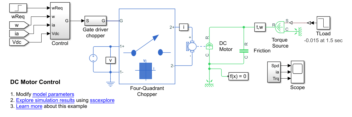
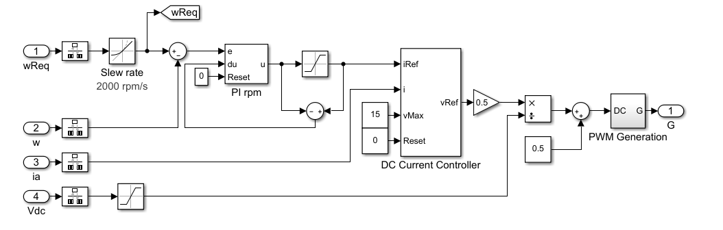
2. The Control subsystem contains the model of the cascaded control system built using blocks from the Simulink^® library.
3. The Four Quadrant Chopper block represents a four-quadrant DC-DC chopper that contains two bridge arms, each of which has two IGBT (Ideal, Switching) blocks. When the input voltage exceeds the threshold of 0.5 V, the IGBT (Ideal, Switching) blocks behave like linear diodes with a forward-voltage of 0.8 V and a resistance of 1e-4 ohm. When the threshold voltage is not exceeded, the IGBT (Ideal, Switching) blocks act like linear resistors with an off-state conductance of 1e-5 1/ohm.
Simulate the model.
```
sim("DCMotorControl")
```
View the results. Open the Scope block.
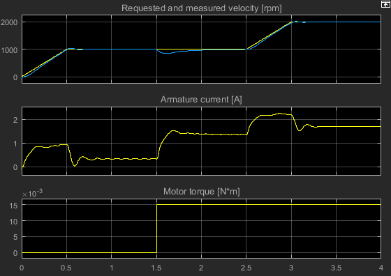
At 1.5 seconds, there is a load torque that results in a steady-state error.
Tune the DC motor controller. The ee_getDCMotorFirstOrderPIParams function calculates the proportional gain, K_P, and the integral gain, K_I, for the first-order system in this example.
The function syntax is [Kp, Ki] = getParamPI(Km,Tm,Ts,sigma,tr).
The input arguments for the function are the system parameters and the requirements for the controller:
- Km is the first-order gain.
- Tm is the time constant of the first-order system.
- T_s is the sample time for the discrete-time controller.
- sigma is the desired maximum overshoot, σ.
- t_r is the desired response time.
♣
1. To examine the equations in the function, enter
  edit ee_getDCMotorFirstOrderPIParams
2. To calculate the controller parameters using the function, save these system parameters to the workspace:
  Ra=4.67; % [Ohm] La=170e-3; % [H] Bm=47.3e-6; % [N*m/(rad/s)] Jm=42.6e-6; % [Kg*m^2] Kb=14.7e-3; % [V/(rad/s)] Tsc=1e-3; % [s]
3. Calculate the parameters for tuning the current controller as a function of the parameters and requirements for the inner controller:
  - Km = 1/Ra.
  - Tm = La/Ra.
  - Ts = Tsc.
  - sigma = 0.05.
  - Tr = 0.11.
  [Kp_i, Ki_i] = ee_getDCMotorFirstOrderPIParams(1/Ra,La/Ra,Tsc,0.05,0.11)
  Kp_i = 7.7099 Ki_i = 455.1491
  The gain parameters for the current controller are saved to the workspace.
4. Calculate the parameters for tuning the speed controller based on the parameters and requirements for the outer controller:
  - Km = Kb*(30/pi).
  - Tm = Jm/Ra.
  - Ts = Tsc.
  - sigma = 0.05.
  - Tr = 0.5.
  [Kp_n, Ki_n] = ee_getDCMotorFirstOrderPIParams((Kb*(30/pi))/Bm,Jm/Bm,Tsc,0.05,0.5)
  Kp_n = 0.0045 Ki_n = 0.0405
The gain parameters for the speed controller are saved to the workspace.
Simulate the model using the saved gain parameters for the speed and controllers.
```
sim("DCMotorControl")
```
View the results. Open the Scope block.

There is slightly more overshoot, however, the controller responds much faster to the load torque change.