Model the Dynamics of Moving Billiard Balls
This example shows how to model the opening shot in a billiards game by using continuous-time matrix variables. In the model, a Stateflow® chart simulates the dynamics of a hybrid system that has a large number of discontinuities. For more information, see Continuous-Time Modeling in Stateflow.
When the simulation starts, a MATLAB® user interface (UI) shows a pool table with 15 billiard balls arranged in a triangular rack. The UI then prompts you to select the initial position and velocity of the cue ball. When the cue ball is released, the UI animates the motion of the billiard balls as they undergo a sequence of rapid collisions.
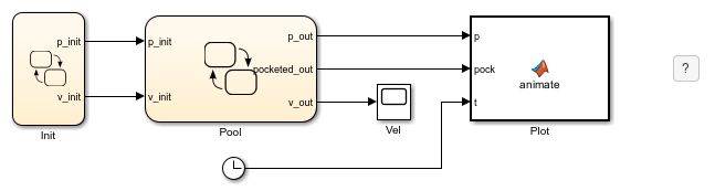
The model consists of:
The Stateflow chart Init, which calls the function
sf_pool_plotter.mto initialize the position and velocity of the cue ball based on the input from the UI.The Stateflow chart Pool, which calculates the two-dimensional dynamics of each billiard ball.
The MATLAB Function block Plot, which calls the function
sf_pool_plotter.mto animate the motion of the billiard balls during the simulation.The Scope block Vel, which displays the velocity of each billiard ball during the opening shot.
Calculate Continuous-Time Dynamics
To represent the dynamics of the billiard balls, the Pool chart makes several assumptions.
Continuous-Time Variables
The chart ignores the spin of the balls, so the state of the system is described completely by the positions and velocities of the balls. Each ball is assumed to have unit mass, so its position and velocity are described by the system of differential equations
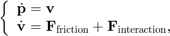
where  and
and  are the forces caused by friction with the pool table and by collisions with other balls.
To track the positions and velocities of the balls, the chart stores a pair of 16-by-2 matrices in the continuous-time variables p and v. In each matrix, the  row represents the two-dimensional position or velocity of the ball.
Friction Model
To calculate the force of friction acting on each ball, the chart calls the MATLAB function frictionForce. This function implements a simplified friction model. Friction acts on each moving ball with a constant force opposite to the direction of motion. Because friction does not act on stationary balls, the force of friction on each ball is inherently modal:

where  is the coefficient of friction and
  is the acceleration due to gravity.
Collision Dynamics
To determine the interactions caused by collisions between balls, the chart calls the MATLAB function interactionForce. This function implements a simple restoring force model when two balls come in contact with each other. The interaction force between the and  balls is modal:
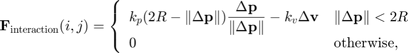
where:
 is the radius of each ball.
 and
and  are constants of elasticity.
 is the relative separation of the centers of the two balls.
 is the relative difference in velocity between the two balls.
Because the balls are free to move in two dimensions, the chart uses the 16-by-16 Boolean matrix ball_interaction to account for all potential collisions. For example, when the and balls are touching, the value of ball_interaction(i,j) is true. Otherwise, this value is false. Because collisions are symmetric in nature, the chart uses only the upper triangular portion of the matrix.
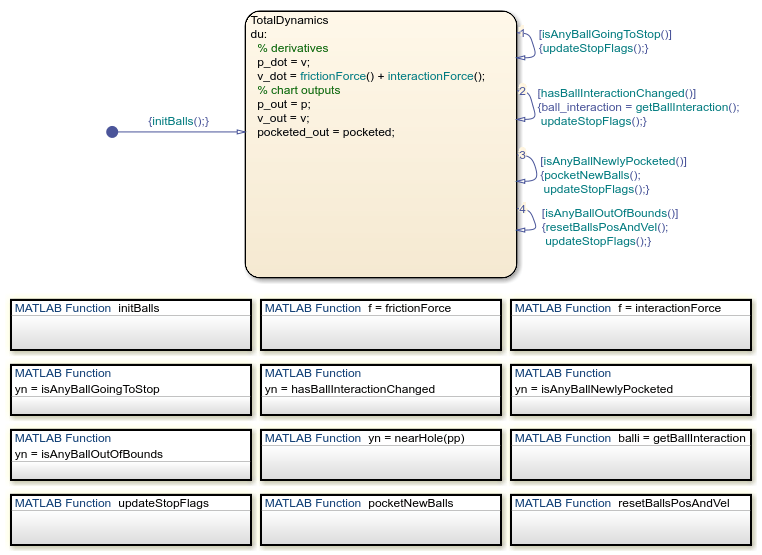
Perform Matrix Calculations in MATLAB Functions
To compute the two-dimensional dynamics of the billiard balls, the Pool chart calls several MATLAB functions that perform matrix calculations.
initBallsinitializes the position and velocity of every ball on the pool table.frictionForcecalculates the friction force acting on each ball.interactionForcecalculates the interaction force acting on each ball.isAnyBallGoingToStopreturns a value of1if any ball stops moving. Otherwise, the function returns a value of0.hasBallInteractionChangedreturns a value of1if any ball interactions change. Otherwise, the function returns a value of0.isAnyBallNewlyPocketedreturns a value of1if any ball falls in a pocket. Otherwise, the function returns a value of0.isAnyBallOutOfBoundsreturns a value oftrueif any ball lies outside the boundary of the pool table. Otherwise, the function returns a value offalse.nearHolereturns a value oftrueif a ball is near a pocket on the pool table. Otherwise, the function returns a value offalse.getBallInteractionreturns a Boolean matrix that specifies whether any balls are in contact with each other.updateStopFlagskeeps track of which balls have stopped moving and stores the result in the vectorstopped.pocketNewBallssets the velocity of each pocketed ball to0.resetBallsPosAndVelresets the position and velocity of any ball that lies outside the boundary of the pool table.
View the Simulation Results
When you start the simulation, a UI shows a pool table with 15 billiard balls arranged at one end of the table. To specify the initial position of the cue ball, click anywhere on the pool table.
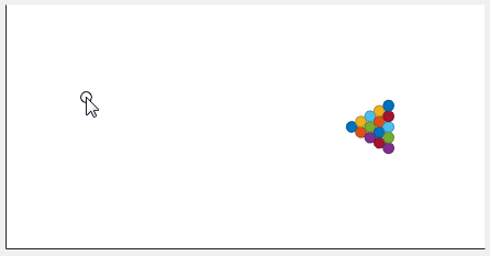
To specify the initial velocity of the cue ball, click a different spot on the pool table.

The model simulates the dynamics of the system and animates the motion of the billiard balls.

To stop the simulation, close the UI.