ANOVA with Random Effects

Set Up the Model

Load the sample data.

load mileage

The anova2 function works only with balanced data, and it infers the values of the grouping variables from the row and column numbers of the input matrix. The anovan function, on the other hand, requires you to explicitly create vectors of grouping variable values. Create these vectors in the following way.

Create an array indicating the factory for each value in mileage. This array is 1 for the first column, 2 for the second, and 3 for the third.

factory  = repmat(1:3,6,1);

Create an array indicating the car model for each mileage value. This array is 1 for the first three rows of mileage, and 2 for the remaining three rows.

carmod = [ones(3,3); 2*ones(3,3)];

Turn these matrices into vectors and display them.

mileage = mileage(:);
factory = factory(:);
carmod = carmod(:);
[mileage factory carmod]

ans = 18×3

   33.3000    1.0000    1.0000
   33.4000    1.0000    1.0000
   32.9000    1.0000    1.0000
   32.6000    1.0000    2.0000
   32.5000    1.0000    2.0000
   33.0000    1.0000    2.0000
   34.5000    2.0000    1.0000
   34.8000    2.0000    1.0000
   33.8000    2.0000    1.0000
   33.4000    2.0000    2.0000
      ⋮

Fit a Random Effects Model

Suppose you are studying a few factories but you want information about what would happen if you build these same car models in a different factory, either one that you already have or another that you might construct. To get this information, fit the analysis of variance model, specifying a model that includes an interaction term and that the factory factor is random.

[pvals,tbl,stats] = anovan(mileage, {factory carmod}, ... 
'model',2, 'random',1,'varnames',{'Factory' 'Car Model'});

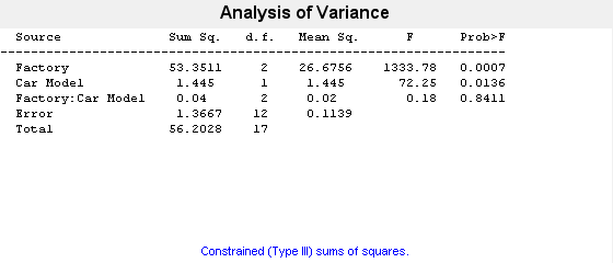
In the fixed effects version of this fit, which you get by omitting the inputs 'random',1 in the preceding code, the effect of car model is significant, with a p-value of 0.0039. But in this example, which takes into account the random variation of the effect of the variable 'Car Model' from one factory to another, the effect is still significant, but with a higher p-value of 0.0136.

F-Statistics for Models with Random Effects

The F-statistic in a model having random effects is defined differently than in a model having all fixed effects. In the fixed effects model, you compute the F-statistic for any term by taking the ratio of the mean square for that term with the mean square for error. In a random effects model, however, some F-statistics use a different mean square in the denominator.

In the example described in Set Up the Model, the effect of the variable 'Factory' could vary across car models. In this case, the interaction mean square takes the place of the error mean square in the F-statistic.

Find the F-statistic.

F = 26.6756 / 0.02

F = 
1.3338e+03

The degrees of freedom for the statistic are the degrees of freedom for the numerator (2) and denominator (2) mean squares.

Find the p-value.

pval = 1 - fcdf(F,2,2)

pval = 
7.4919e-04

With random effects, the expected value of each mean square depends not only on the variance of the error term, but also on the variances contributed by the random effects. You can see these dependencies by writing the expected values as linear combinations of contributions from the various model terms.

Find the coefficients of these linear combinations.

stats.ems

ans = 4×4

    6.0000    0.0000    3.0000    1.0000
    0.0000    9.0000    3.0000    1.0000
    0.0000    0.0000    3.0000    1.0000
         0         0         0    1.0000

This returns the ems field of the stats structure.

Display text representations of the linear combinations.

stats.txtems

ans = 4x1 cell
    {'6*V(Factory)+3*V(Factory:Car Model)+V(Error)'  }
    {'9*Q(Car Model)+3*V(Factory:Car Model)+V(Error)'}
    {'3*V(Factory:Car Model)+V(Error)'               }
    {'V(Error)'                                      }

The expected value for the mean square due to car model (second term) includes contributions from a quadratic function of the car model effects, plus three times the variance of the interaction term's effect, plus the variance of the error term. Notice that if the car model effects were all zero, the expression would reduce to the expected mean square for the third term (the interaction term). That is why the F-statistic for the car model effect uses the interaction mean square in the denominator.

In some cases there is no single term whose expected value matches the one required for the denominator of the F-statistic. In that case, the denominator is a linear combination of mean squares. The stats structure contains fields giving the definitions of the denominators for each F-statistic. The txtdenom field, stats.txtdenom, contains a text representation, and the denom field contains a matrix that defines a linear combination of the variances of terms in the model. For balanced models like this one, the denom matrix, stats.denom, contains zeros and ones, because the denominator is just a single term's mean square.

Display the txtdenom field.

stats.txtdenom

ans = 3x1 cell
    {'MS(Factory:Car Model)'}
    {'MS(Factory:Car Model)'}
    {'MS(Error)'            }

Display the denom field.

stats.denom

ans = 3×3

    0.0000    1.0000    0.0000
    0.0000    1.0000    0.0000
   -0.0000    0.0000    1.0000

Variance Components

For the model described in Set Up the Model, consider the mileage for a particular car of a particular model made at a random factory. The variance of that car is the sum of components, or contributions, one from each of the random terms.

Display the names of the random terms.

stats.rtnames

ans = 3x1 cell
    {'Factory'          }
    {'Factory:Car Model'}
    {'Error'            }

You do not know the variances, but you can estimate them from the data. Recall that the ems field of the stats structure expresses the expected value of each term's mean square as a linear combination of unknown variances for random terms, and unknown quadratic forms for fixed terms. If you take the expected mean square expressions for the random terms, and equate those expected values to the computed mean squares, you get a system of equations that you can solve for the unknown variances. These solutions are the variance component estimates.

Display the variance component estimate for each term.

stats.varest

ans = 3×1

    4.4426
   -0.0313
    0.1139

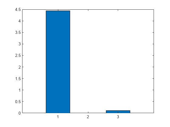
Under some conditions, the variability attributed to a term is unusually low, and that term's variance component estimate is negative. In those cases it is common to set the estimate to zero, which you might do, for example, to create a bar graph of the components.

Create a bar graph of the components.

bar(max(0,stats.varest))

gca.xtick = 1:3;
gca.xticklabel = stats.rtnames;

You can also compute confidence bounds for the variance estimate. The anovan function does this by computing confidence bounds for the variance expected mean squares, and finding lower and upper limits on each variance component containing all of these bounds. This procedure leads to a set of bounds that is conservative for balanced data. (That is, 95% confidence bounds will have a probability of at least 95% of containing the true variances if the number of observations for each combination of grouping variables is the same.) For unbalanced data, these are approximations that are not guaranteed to be conservative.

Display the variance estimates and the confidence limits for the variance estimates of each component.

[{'Term' 'Estimate' 'Lower' 'Upper'};
 stats.rtnames, num2cell([stats.varest stats.varci])]

ans=4×4 cell array
    {'Term'             }    {'Estimate'}    {'Lower' }    {'Upper'   }
    {'Factory'          }    {[  4.4426]}    {[1.0736]}    {[175.6038]}
    {'Factory:Car Model'}    {[ -0.0313]}    {[   NaN]}    {[     NaN]}
    {'Error'            }    {[  0.1139]}    {[0.0586]}    {[  0.3103]}