residuals

Residuals of fitted linear mixed-effects model

Syntax

R = residuals(lme)

R = residuals(lme,Name,Value)

Description

R = residuals(lme) returns the raw conditional residuals from a fitted linear mixed-effects model lme.

R = residuals(lme,Name,Value) returns the residuals from the linear mixed-effects model lme with additional options specified by one or more Name,Value pair arguments.

For example, you can specify Pearson or standardized residuals, or residuals with contributions from only fixed effects.

example

Examples

collapse all

Plot Residuals vs. Fitted Values

Open Live Script

Load the sample data.

load('weight.mat');

weight contains data from a longitudinal study, where 20 subjects are randomly assigned to 4 exercise programs, and their weight loss is recorded over six 2-week time periods. This is simulated data.

Store the data in a table. Define Subject and Program as categorical variables.

tbl = table(InitialWeight,Program,Subject,Week,y);
tbl.Subject = nominal(tbl.Subject);
tbl.Program = nominal(tbl.Program);

Fit a linear mixed-effects model where the initial weight, type of program, week, and the interaction between the week and type of program are the fixed effects. The intercept and week vary by subject.

lme = fitlme(tbl,'y ~ InitialWeight + Program*Week + (Week|Subject)');

Compute the fitted values and raw residuals.

F = fitted(lme);
R = residuals(lme);

Plot the residuals versus the fitted values.

plot(F,R,'bx')
xlabel('Fitted Values')
ylabel('Residuals')

Figure contains an axes object. The axes object with xlabel Fitted Values, ylabel Residuals contains a line object which displays its values using only markers.

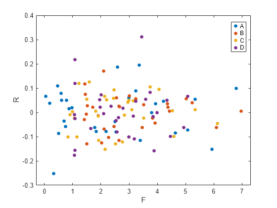
Now, plot the residuals versus the fitted values, grouped by program.

figure();
gscatter(F,R,Program)

Figure contains an axes object. The axes object with xlabel F, ylabel R contains 4 objects of type line. One or more of the lines displays its values using only markers These objects represent A, B, C, D.

The residuals seem to behave similarly across levels of the program as expected.

Compute Conditional and Marginal Pearson Residuals

Open Live Script

Load the sample data.

load carbig

Store the variables for miles per gallon (MPG), acceleration, horsepower, cylinders, and model year in a table.

tbl = table(MPG,Acceleration,Horsepower,Cylinders,Model_Year);

Fit a linear mixed-effects model for miles per gallon (MPG), with fixed effects for acceleration, horsepower, and the cylinders, and potentially correlated random effects for intercept and acceleration grouped by model year.

lme = fitlme(tbl,'MPG ~ Acceleration + Horsepower + Cylinders + (Acceleration|Model_Year)');

Compute the conditional Pearson residuals and display the first five residuals.

PR = residuals(lme,'ResidualType','Pearson');
PR(1:5)

Compute the marginal Pearson residuals and display the first five residuals.

PRM = residuals(lme,'ResidualType','Pearson','Conditional',false);
PRM(1:5)

Examine Residuals

Open Live Script

Load the sample data.

load carbig

Store the variables for miles per gallon (MPG), acceleration, horsepower, cylinders, and model year in a table.

tbl = table(MPG,Acceleration,Horsepower,Cylinders,Model_Year);

lme = fitlme(tbl,'MPG ~ Acceleration + Horsepower + Cylinders + (Acceleration|Model_Year)');

Draw a histogram of the raw residuals with a normal fit.

r = residuals(lme);
histfit(r)

Figure contains an axes object. The axes object contains 2 objects of type bar, line.

Normal distribution seems to be a good fit for the residuals.

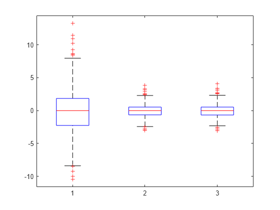
Compute the conditional Pearson and standardized residuals and create box plots of all three types of residuals.

pr = residuals(lme,'ResidualType','Pearson');
st = residuals(lme,'ResidualType','Standardized');
X = [r pr st];
boxplot(X)

Figure contains an axes object. The axes object contains 21 objects of type line. One or more of the lines displays its values using only markers

Red plus signs show the observations with residuals above or below $q 3 + 1.5 (q 3 - q 1)$ and $q 1 - 1.5 (q 3 - q 1)$ , where $q 1$ and $q 3$ are the 25th and 75th percentiles, respectively.

Find the observations with residuals that are 2.5 standard deviations above and below the mean.

find(r > mean(r,'omitnan') + 2.5*std(r,'omitnan'))

find(r < mean(r,'omitnan') - 2.5*std(r,'omitnan'))

Input Arguments

collapse all

`lme` — Linear mixed-effects model
`LinearMixedModel` object

Linear mixed-effects model, specified as a LinearMixedModel object constructed using fitlme or fitlmematrix.

Name-Value Arguments

Specify optional pairs of arguments as Name1=Value1,...,NameN=ValueN, where Name is the argument name and Value is the corresponding value. Name-value arguments must appear after other arguments, but the order of the pairs does not matter.

Before R2021a, use commas to separate each name and value, and enclose Name in quotes.

Example: R = residuals(lme,'ResidualType','Pearson');

`Conditional` — Indicator for conditional residuals
`True` (default) | `False`

Indicator for conditional residuals, specified as the comma-separated pair consisting of 'Conditional' and one of the following.

`True`	Contribution from both fixed effects and random effects (conditional)
`False`	Contribution from only fixed effects (marginal)

Example: 'Conditional,'False'

`ResidualType` — Residual type
`'Raw'` (default) | `'Pearson'` | `'Standardized'`

Residual type, specified by the comma-separated pair consisting of ResidualType and one of the following.

Residual Type Conditional Marginal

Residual Type	Conditional	Marginal
`'Raw'`	$r_{i}^{C} = {[y - X \hat{β} - Z \hat{b}]}_{i}$	$r_{i}^{M} = {[y - X \hat{β}]}_{i}$
`'Pearson'`	$p r_{i}^{C} = \frac{r_{i}^{C}}{{\sqrt{[{\hat{V a r}}_{y, b} (y - X β - Z b)]}}_{i i}}$	$p r_{i}^{M} = \frac{r_{i}^{M}}{\sqrt{{[{\hat{V a r}}_{y} (y - X β)]}_{i i}}}$
`'Standardized'`	$s t_{i}^{C} = \frac{r_{i}^{C}}{\sqrt{{[{\hat{V a r}}_{y} (r^{C})]}_{i i}}}$	$s t_{i}^{M} = \frac{r_{i}^{M}}{\sqrt{{[{\hat{V a r}}_{y} (r^{M})]}_{i i}}}$

'Raw'

$r_{i}^{C} = {[y - X \hat{β} - Z \hat{b}]}_{i}$

$r_{i}^{M} = {[y - X \hat{β}]}_{i}$

'Pearson'

$p r_{i}^{C} = \frac{r_{i}^{C}}{{\sqrt{[{\hat{V a r}}_{y, b} (y - X β - Z b)]}}_{i i}}$

$p r_{i}^{M} = \frac{r_{i}^{M}}{\sqrt{{[{\hat{V a r}}_{y} (y - X β)]}_{i i}}}$

'Standardized'

$s t_{i}^{C} = \frac{r_{i}^{C}}{\sqrt{{[{\hat{V a r}}_{y} (r^{C})]}_{i i}}}$

$s t_{i}^{M} = \frac{r_{i}^{M}}{\sqrt{{[{\hat{V a r}}_{y} (r^{M})]}_{i i}}}$

For more information on the conditional and marginal residuals and residual variances, see Definitions at the end of this page.

Example: 'ResidualType','Standardized'

Output Arguments

collapse all

`R` — Residuals
n-by-1 vector

Residuals of the fitted linear mixed-effects model lme returned as an n-by-1 vector, where n is the number of observations.

More About

collapse all

Conditional and Marginal Residuals

Conditional residuals include contributions from both fixed and random effects, whereas marginal residuals include contribution from only fixed effects.

Suppose the linear mixed-effects model lmehas an n-by-p fixed-effects design matrix X and an n-by-q random-effects design matrix Z. Also, suppose the p-by-1 estimated fixed-effects vector is $\hat{β}$ , and the q-by-1 estimated best linear unbiased predictor (BLUP) vector of random effects is $\hat{b}$ . The fitted conditional response is

${\hat{y}}_{C o n d} = X \hat{β} + Z \hat{b},$

and the fitted marginal response is

${\hat{y}}_{M a r} = X \hat{β},$

residuals can return three types of residuals: raw, Pearson, and standardized. For any type, you can compute the conditional or the marginal residuals. For example, the conditional raw residual is

$r_{C o n d} = y - X \hat{β} - Z \hat{b},$

and the marginal raw residual is

$r_{M a r} = y - X \hat{β} .$

For more information on other types of residuals, see the ResidualType name-value pair argument.

Version History

Introduced in R2013b

residuals

Syntax

Description

Examples

Plot Residuals vs. Fitted Values

Compute Conditional and Marginal Pearson Residuals

Examine Residuals

Input Arguments

lme — Linear mixed-effects model LinearMixedModel object

Name-Value Arguments

Conditional — Indicator for conditional residuals True (default) | False

ResidualType — Residual type 'Raw' (default) | 'Pearson' | 'Standardized'

Output Arguments

R — Residuals n-by-1 vector

More About

Conditional and Marginal Residuals

Version History

See Also

`lme` — Linear mixed-effects model
`LinearMixedModel` object

`Conditional` — Indicator for conditional residuals
`True` (default) | `False`

`ResidualType` — Residual type
`'Raw'` (default) | `'Pearson'` | `'Standardized'`

`R` — Residuals
n-by-1 vector