Predict Class Labels Using ClassificationEnsemble Predict Block
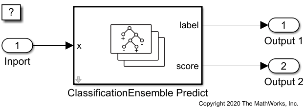
This example shows how to train an ensemble model with optimal hyperparameters, and then use the ClassificationEnsemble Predict block for label prediction in Simulink®. The block accepts an observation (predictor data) and returns the predicted class label and class score for the observation using the trained classification ensemble model.
Train Classification Model with Optimal Hyperparameters
Load the CreditRating_Historical data set. This data set contains customer IDs and their financial ratios, industry labels, and credit ratings. Determine the sample size.
tbl = readtable('CreditRating_Historical.dat');
n = numel(tbl)
n = 31456
Display the first three rows of the table.
head(tbl,3)
     ID      WC_TA    RE_TA    EBIT_TA    MVE_BVTD    S_TA     Industry    Rating
    _____    _____    _____    _______    ________    _____    ________    ______

    62394    0.013    0.104     0.036      0.447      0.142       3        {'BB'}
    48608    0.232    0.335     0.062      1.969      0.281       8        {'A' }
    42444    0.311    0.367     0.074      1.935      0.366       1        {'A' }
tbl.Industry is a categorical variable for an industry label. When you train a model for the ClassificationEnsemble Predict block, you must preprocess categorical predictors by using the dummyvar function to include the categorical predictors in the model. You cannot use the 'CategoricalPredictors' name-value argument. Create dummy variables for tbl.Industry.
d = dummyvar(tbl.Industry);
dummyvar creates dummy variables for each category of tbl.Industry. Determine the number of categories in tbl.Industry and the number of dummy variables in d.
unique(tbl.Industry)'
ans = 1×12

     1     2     3     4     5     6     7     8     9    10    11    12
size(d)
ans = 1×2

        3932          12
Create a numeric matrix for the predictor variables and a cell array for the response variable.
X = [table2array(tbl(:,2:6)) d];
Y = tbl.Rating;
X is a numeric matrix that contains 17 variables: the five financial ratios and the 12 dummy variables for the industry label. X does not use tbl.ID because the variable is not helpful in predicting credit ratings. Y is a cell array of character vectors that contains the corresponding credit ratings.
Suppose that you receive the data in sequence, and you have the first 3000 observations, but you have not received the last 932 yet. Partition the data into present and future samples.
prsntX = X(1:3000,:);
prsntY = Y(1:3000);
ftrX = X(3001:end,:);
ftrY = Y(3001:end);
Train an ensemble using all presently available data prsntX and prsntY with these options:
Specify
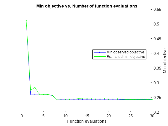
'OptimizeHyperparameters'as'auto'to train an ensemble with optimal hyperparameters. The'auto'option finds optimal values for'Method','NumLearningCycles', and'LearnRate'(for applicable methods) offitcensembleand'MinLeafSize'of tree learners.For reproducibility, set the random seed and use the
'expected-improvement-plus'acquisition function. Also, for reproducibility of the random forest algorithm, specify'Reproducible'astruefor tree learners.Specify the order of the classes by using the
'ClassNames'name-value argument. The output values from the score port of the ClassificationEnsemble Predict block have the same order.
rng('default')
t = templateTree('Reproducible',true);
ensMdl = fitcensemble(prsntX,prsntY, ...
    'ClassNames',{'AAA' 'AA' 'A' 'BBB' 'BB' 'B' 'CCC'}, ...
    'OptimizeHyperparameters','auto','Learners',t, ...
    'HyperparameterOptimizationOptions', ...
    struct('AcquisitionFunctionName','expected-improvement-plus'))
|===================================================================================================================================|
| Iter | Eval   | Objective   | Objective   | BestSoFar   | BestSoFar   |       Method | NumLearningC-|    LearnRate |  MinLeafSize |
|      | result |             | runtime     | (observed)  | (estim.)    |              | ycles        |              |              |
|===================================================================================================================================|
|    1 | Best   |     0.51133 |       15.97 |     0.51133 |     0.51133 |   AdaBoostM2 |          429 |     0.082478 |          871 |
|    2 | Best   |     0.26133 |      23.171 |     0.26133 |     0.27463 |   AdaBoostM2 |          492 |      0.19957 |            4 |
|    3 | Accept |     0.85133 |     0.83994 |     0.26133 |     0.28421 |     RUSBoost |           10 |      0.34528 |         1179 |
|    4 | Accept |       0.263 |     0.77678 |     0.26133 |     0.26124 |   AdaBoostM2 |           13 |      0.27107 |           10 |
|    5 | Best   |        0.26 |       1.247 |        0.26 |     0.26003 |          Bag |           10 |            - |            1 |
|    6 | Accept |     0.28933 |      1.8886 |        0.26 |      0.2602 |          Bag |           36 |            - |          101 |
|    7 | Best   |     0.25667 |       1.735 |     0.25667 |     0.25726 |   AdaBoostM2 |           33 |      0.99501 |           11 |
|    8 | Best   |       0.244 |      32.962 |       0.244 |     0.24406 |          Bag |          460 |            - |            7 |
|    9 | Accept |       0.246 |      4.7119 |       0.244 |     0.24435 |          Bag |           60 |            - |            4 |
|   10 | Accept |     0.25533 |      1.7242 |       0.244 |     0.24437 |   AdaBoostM2 |           33 |      0.99516 |            1 |
|   11 | Accept |     0.25733 |       1.898 |       0.244 |      0.2442 |          Bag |           25 |            - |            8 |
|   12 | Accept |     0.74267 |      18.987 |       0.244 |     0.24449 |          Bag |          498 |            - |         1462 |
|   13 | Accept |     0.28433 |      10.744 |       0.244 |     0.24621 |     RUSBoost |          210 |    0.0011248 |            1 |
|   14 | Accept |     0.25733 |      25.844 |       0.244 |     0.24555 |          Bag |          488 |            - |           32 |
|   15 | Accept |     0.28567 |     0.66833 |       0.244 |     0.24554 |     RUSBoost |           11 |      0.18108 |            6 |
|   16 | Accept |     0.25133 |      21.788 |       0.244 |     0.24547 |   AdaBoostM2 |          474 |      0.15161 |           43 |
|   17 | Accept |     0.24567 |      37.148 |       0.244 |     0.24459 |          Bag |          490 |            - |            3 |
|   18 | Accept |     0.26033 |      21.358 |       0.244 |      0.2449 |   AdaBoostM2 |          472 |     0.017039 |           24 |
|   19 | Accept |     0.28467 |      1.0004 |       0.244 |     0.24561 |     RUSBoost |           19 |      0.95267 |            2 |
|   20 | Best   |       0.244 |      35.361 |       0.244 |     0.24454 |          Bag |          486 |            - |            3 |
|===================================================================================================================================|
| Iter | Eval   | Objective   | Objective   | BestSoFar   | BestSoFar   |       Method | NumLearningC-|    LearnRate |  MinLeafSize |
|      | result |             | runtime     | (observed)  | (estim.)    |              | ycles        |              |              |
|===================================================================================================================================|
|   21 | Accept |        0.26 |      1.0501 |       0.244 |     0.24458 |   AdaBoostM2 |           20 |      0.88583 |           35 |
|   22 | Accept |     0.24733 |      31.308 |       0.244 |     0.24487 |          Bag |          448 |            - |            5 |
|   23 | Best   |     0.24333 |      36.065 |     0.24333 |     0.24427 |          Bag |          497 |            - |            3 |
|   24 | Accept |     0.24333 |      38.869 |     0.24333 |     0.24374 |          Bag |          499 |            - |            2 |
|   25 | Accept |     0.24367 |      36.523 |     0.24333 |     0.24366 |          Bag |          482 |            - |            2 |
|   26 | Accept |       0.257 |      21.389 |     0.24333 |     0.24364 |   AdaBoostM2 |          487 |      0.72228 |           85 |
|   27 | Accept |     0.31167 |      19.351 |     0.24333 |     0.24372 |     RUSBoost |          445 |     0.012747 |          101 |
|   28 | Accept |     0.32033 |      23.955 |     0.24333 |     0.24386 |     RUSBoost |          487 |      0.82301 |           31 |
|   29 | Accept |       0.244 |      39.404 |     0.24333 |     0.24372 |          Bag |          476 |            - |            2 |
|   30 | Accept |       0.261 |     0.93501 |     0.24333 |     0.24367 |          Bag |           10 |            - |            2 |

__________________________________________________________
Optimization completed.
MaxObjectiveEvaluations of 30 reached.
Total function evaluations: 30
Total elapsed time: 518.9828 seconds
Total objective function evaluation time: 508.672

Best observed feasible point:
    Method    NumLearningCycles    LearnRate    MinLeafSize
    ______    _________________    _________    ___________

     Bag             497              NaN            3

Observed objective function value = 0.24333
Estimated objective function value = 0.24424
Function evaluation time = 36.0653

Best estimated feasible point (according to models):
    Method    NumLearningCycles    LearnRate    MinLeafSize
    ______    _________________    _________    ___________

     Bag             499              NaN            2

Estimated objective function value = 0.24367
Estimated function evaluation time = 38.7372
ensMdl =
  ClassificationBaggedEnsemble
                         ResponseName: 'Y'
                CategoricalPredictors: []
                           ClassNames: {'AAA'  'AA'  'A'  'BBB'  'BB'  'B'  'CCC'}
                       ScoreTransform: 'none'
                      NumObservations: 3000
    HyperparameterOptimizationResults: [1×1 BayesianOptimization]
                           NumTrained: 499
                               Method: 'Bag'
                         LearnerNames: {'Tree'}
                 ReasonForTermination: 'Terminated normally after completing the requested number of training cycles.'
                              FitInfo: []
                   FitInfoDescription: 'None'
                            FResample: 1
                              Replace: 1
                     UseObsForLearner: [3000×499 logical]


  Properties, Methods
fitcensemble returns a ClassificationBaggedEnsemble object because the function finds the random forest algorithm ('Bag') as the optimal method.
Create Simulink Model
This example provides the Simulink model slexCreditRatingClassificationEnsemblePredictExample.slx, which includes the ClassificationEnsemble Predict block. You can open the Simulink model or create a new model as described in this section.
Open the Simulink model slexCreditRatingClassificationEnsemblePredictExample.slx.
SimMdlName = 'slexCreditRatingClassificationEnsemblePredictExample';
open_system(SimMdlName)
If you open the Simulink model, then the software runs the code in the PreLoadFcn callback function before loading the Simulink model. The PreLoadFcn callback function of slexCreditRatingClassificationEnsemblePredictExample includes code to check if your workspace contains the ensMdl variable for the trained model. If the workspace does not contain the variable, PreLoadFcn loads the sample data, trains the model using the optimal hyperparameters, and creates an input signal for the Simulink model. To view the callback function, in the Setup section on the Modeling tab, click Model Settings and select Model Properties. Then, on the Callbacks tab, select the PreLoadFcn callback function in the Model callbacks pane.
To create a new Simulink model, open the Blank Model template and add the ClassificationEnsemble Predict block. Add the Inport and Outport blocks and connect them to the ClassificationEnsemble Predict block.
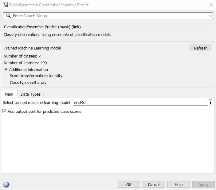
Double-click the ClassificationEnsemble Predict block to open the Block Parameters dialog box. Specify the Select trained machine learning model parameter as ensMdl, which is the name of a workspace variable that contains the trained model. Click the Refresh button. The dialog box displays the options used to train the model ensMdl under Trained Machine Learning Model. Select the Add output port for predicted class scores check box to add the second output port score.

The ClassificationEnsemble Predict block expects an observation containing 17 predictor values. Double-click the Inport block, and set the Port dimensions to 17 on the Signal Attributes tab.
Create an input signal in the form of a structure array for the Simulink model. The structure array must contain these fields:
time— The points in time at which the observations enter the model. In this example, the duration includes the integers from 0 through 931. The orientation must correspond to the observations in the predictor data. So, in this case,timemust be a column vector.signals— A 1-by-1 structure array describing the input data and containing the fieldsvaluesanddimensions, wherevaluesis a matrix of predictor data, anddimensionsis the number of predictor variables.
Create an appropriate structure array for future samples.
creditRatingInput.time = (0:931)';
creditRatingInput.signals(1).values = ftrX;
creditRatingInput.signals(1).dimensions = size(ftrX,2);
To import signal data from the workspace:
Open the Configuration Parameters dialog box. On the Modeling tab, click Model Settings.
In the Data Import/Export pane, select the Input check box and enter
creditRatingInputin the adjacent text box.In the Solver pane, under Simulation time, set Stop time to
creditRatingInput.time(end). Under Solver selection, set Type toFixed-step, and set Solver todiscrete (no continuous states).
For more details, see Load Signal Data for Simulation (Simulink).
Simulate the model.
sim(SimMdlName);
When the Inport block detects an observation, it directs the observation into the ClassificationEnsemble Predict block. You can use the Simulation Data Inspector (Simulink) to view the logged data of the Outport blocks.
See Also
ClassificationEnsemble Predict