Statistics and Machine Learning with Big Data Using Tall Arrays
This example shows how to perform statistical analysis and machine learning on out-of-memory data with MATLAB® and Statistics and Machine Learning Toolbox™.
Tall arrays and tables are designed for working with out-of-memory data. This type of data consists of a very large number of rows (observations) compared to a smaller number of columns (variables). Instead of writing specialized code that takes into account the huge size of the data, such as with MapReduce, you can use tall arrays to work with large data sets in a manner similar to in-memory MATLAB arrays. The fundamental difference is that tall arrays typically remain unevaluated until you request that the calculations be performed.
When you perform calculations on tall arrays, MATLAB® uses either a parallel pool (default if you have Parallel Computing Toolbox™) or the local MATLAB session. To run the example using the local MATLAB session when you have Parallel Computing Toolbox, change the global execution environment by using the mapreducer function.
mapreducer(0)
This example works with a subset of data on a single computer to develop a linear regression model, and then it scales up to analyze all of the data set. You can scale up this analysis even further to:
Work with data that cannot be read into memory
Work with data distributed across clusters using MATLAB Parallel Server™
Integrate with big data systems like Hadoop® and Spark®
Introduction to Machine Learning with Tall Arrays
Several unsupervised and supervised learning algorithms in Statistics and Machine Learning Toolbox are available to work with tall arrays to perform data mining and predictive modeling with out-of-memory data. These algorithms are appropriate for out-of-memory data and can include slight variations from the in-memory algorithms. Capabilities include:
k-Means clustering
Linear regression
Generalized linear regression
Logistic regression
Discriminant analysis
The machine learning workflow for out-of-memory data in MATLAB is similar to in-memory data:
Preprocess
Explore
Develop model
Validate model
Scale up to larger data
This example follows a similar structure in developing a predictive model for airline delays. The data includes a large file of airline flight information from 1987 through 2008. The example goal is to predict the departure delay based on a number of variables.
Details on the fundamental aspects of tall arrays are included in the example Analyze Big Data in MATLAB Using Tall Arrays. This example extends the analysis to include machine learning with tall arrays.
Create Tall Table of Airline Data
A datastore is a repository for collections of data that are too large to fit in memory. You can create a datastore from a number of different file formats as the first step to create a tall array from an external data source.
Create a datastore for the sample file airlinesmall.csv. Select the variables of interest, treat 'NA' values as missing data, and generate a preview table of the data.
ds = datastore('airlinesmall.csv');
ds.SelectedVariableNames = {'Year','Month','DayofMonth','DayOfWeek',...
    'DepTime','ArrDelay','DepDelay','Distance'};
ds.TreatAsMissing = 'NA';
pre = preview(ds)
pre=8×8 table
    Year    Month    DayofMonth    DayOfWeek    DepTime    ArrDelay    DepDelay    Distance
    ____    _____    __________    _________    _______    ________    ________    ________

    1987     10          21            3          642          8          12         308
    1987     10          26            1         1021          8           1         296
    1987     10          23            5         2055         21          20         480
    1987     10          23            5         1332         13          12         296
    1987     10          22            4          629          4          -1         373
    1987     10          28            3         1446         59          63         308
    1987     10           8            4          928          3          -2         447
    1987     10          10            6          859         11          -1         954
Create a tall table backed by the datastore to facilitate working with the data. The underlying data type of a tall array depends on the type of datastore. In this case, the datastore is tabular text and returns a tall table. The display includes a preview of the data, with indication that the size is unknown.
tt = tall(ds)
tt =

  M×8 tall table

    Year    Month    DayofMonth    DayOfWeek    DepTime    ArrDelay    DepDelay    Distance
    ____    _____    __________    _________    _______    ________    ________    ________

    1987     10          21            3          642          8          12         308
    1987     10          26            1         1021          8           1         296
    1987     10          23            5         2055         21          20         480
    1987     10          23            5         1332         13          12         296
    1987     10          22            4          629          4          -1         373
    1987     10          28            3         1446         59          63         308
    1987     10           8            4          928          3          -2         447
    1987     10          10            6          859         11          -1         954
     :        :          :             :           :          :           :           :
     :        :          :             :           :          :           :           :
Preprocess Data
This example aims to explore the time of day and day of week in more detail. Convert the day of week to categorical data with labels and determine the hour of day from the numeric departure time variable.
tt.DayOfWeek = categorical(tt.DayOfWeek,1:7,{'Sun','Mon','Tues',...
    'Wed','Thu','Fri','Sat'});
tt.Hr = discretize(tt.DepTime,0:100:2400,0:23)
tt =
M×9 tall table
Year Month DayofMonth DayOfWeek DepTime ArrDelay DepDelay Distance Hr
____ _____ __________ _________ _______ ________ ________ ________ __
1987 10 21 Tues 642 8 12 308 6
1987 10 26 Sun 1021 8 1 296 10
1987 10 23 Thu 2055 21 20 480 20
1987 10 23 Thu 1332 13 12 296 13
1987 10 22 Wed 629 4 -1 373 6
1987 10 28 Tues 1446 59 63 308 14
1987 10 8 Wed 928 3 -2 447 9
1987 10 10 Fri 859 11 -1 954 8
: : : : : : : : :
: : : : : : : : :
Include only years after 2000 and ignore rows with missing data. Identify data of interest by logical condition.
idx = tt.Year >= 2000 & ...
    ~any(ismissing(tt),2);
tt = tt(idx,:);
Explore Data by Group
A number of exploratory functions are available for tall arrays. For example, the grpstats function calculates grouped statistics of tall arrays. Explore the data by determining the centrality and spread of the data with summary statistics grouped by day of week. Also, explore the correlation between the departure delay and arrival delay.
g = grpstats(tt(:,{'ArrDelay','DepDelay','DayOfWeek'}),'DayOfWeek',...
    {'mean','std','skewness','kurtosis'})
g =
M×11 tall table
GroupLabel DayOfWeek GroupCount mean_ArrDelay std_ArrDelay skewness_ArrDelay kurtosis_ArrDelay mean_DepDelay std_DepDelay skewness_DepDelay kurtosis_DepDelay
__________ _________ __________ _____________ ____________ _________________ _________________ _____________ ____________ _________________ _________________
? ? ? ? ? ? ? ? ? ? ?
? ? ? ? ? ? ? ? ? ? ?
? ? ? ? ? ? ? ? ? ? ?
: : : : : : : : : : :
: : : : : : : : : : :
Preview deferred. Learn more.
C = corr(tt.DepDelay,tt.ArrDelay)
C =

  M×N×... tall array

    ?    ?    ?    ...
    ?    ?    ?    ...
    ?    ?    ?    ...
    :    :    :
    :    :    :

Preview deferred. Learn more.
These commands produce more tall arrays. The commands are not executed until you explicitly gather the results into the workspace. The gather command triggers execution and attempts to minimize the number of passes required through the data to perform the calculations. gather requires that the resulting variables fit into memory.
[statsByDay,C] = gather(g,C)
Evaluating tall expression using the Local MATLAB Session:
- Pass 1 of 1: Completed in 0.77 sec
Evaluation completed in 1.2 sec
statsByDay=7×11 table
    GroupLabel    DayOfWeek    GroupCount    mean_ArrDelay    std_ArrDelay    skewness_ArrDelay    kurtosis_ArrDelay    mean_DepDelay    std_DepDelay    skewness_DepDelay    kurtosis_DepDelay
    __________    _________    __________    _____________    ____________    _________________    _________________    _____________    ____________    _________________    _________________

     {'Fri' }       Fri           7339          4.1512             32.1             7.082               120.53             7.0857           29.339            8.9387               168.37
     {'Mon' }       Mon           8443          5.2487           32.453            4.5811               37.175             6.8319           28.573            5.6468               50.271
     {'Sat' }       Sat           8045           7.132           33.108            3.6457               22.991             9.1557           29.731            4.5135               31.228
     {'Sun' }       Sun           8570          7.7515           36.003            5.7943                80.91             9.3324           32.516            7.2146               118.25
     {'Thu' }       Thu           8601          10.053            36.18            4.1381               37.051             10.923           34.708            1.1414               138.38
     {'Tues'}       Tues          8381          6.4786           32.322             4.374               38.694             7.6083           28.394            5.2012               46.249
     {'Wed' }       Wed           8489          9.3324           37.406            5.1638               57.479                 10           33.426            6.4336               85.426
C =
0.8966
The variables containing the results are now in-memory variables in the Workspace. Based on these calculations, variation occurs in the data and there is correlation between the delays that you can investigate further.
Explore the effect of day of week and hour of day and gain additional statistical information such as the standard error of the mean and the 95% confidence interval for the mean. You can pass the entire tall table and specify which variables to perform calculations on.
byDayHr = grpstats(tt,{'Hr','DayOfWeek'},...
    {'mean','sem','meanci'},'DataVar','DepDelay');
byDayHr = gather(byDayHr);
Evaluating tall expression using the Local MATLAB Session: - Pass 1 of 1: Completed in 0.54 sec Evaluation completed in 0.7 sec
Due to the data partitioning of the tall array, the output might be unordered. Rearrange the data in memory for further exploration.
x = unstack(byDayHr(:,{'Hr','DayOfWeek','mean_DepDelay'}),...
    'mean_DepDelay','DayOfWeek');
x = sortrows(x)x=24×8 table
Hr Sun Mon Tues Wed Thu Fri Sat
__ _______ ________ ________ _______ _______ _______ _______
0 38.519 71.914 39.656 34.667 90 25.536 65.579
1 45.846 27.875 93.6 125.23 52.765 38.091 29.182
2 NaN 39 102 NaN 78.25 -1.5 NaN
3 NaN NaN NaN NaN -377.5 53.5 NaN
4 -7 -6.2857 -7 -7.3333 -10.5 -5 NaN
5 -2.2409 -3.7099 -4.0146 -3.9565 -3.5897 -3.5766 -4.1474
6 0.4 -1.8909 -1.9802 -1.8304 -1.3578 0.84161 -2.2537
7 3.4173 -0.47222 -0.18893 0.71546 0.08 1.069 -1.3221
8 2.3759 1.4054 1.6745 2.2345 2.9668 1.6727 0.88213
9 2.5325 1.6805 2.7656 2.683 5.6138 3.4838 2.5011
10 6.37 5.2868 3.6822 7.5773 5.3372 6.9391 4.9979
11 6.9946 4.9165 5.5639 5.5936 7.0435 4.8989 5.2839
12 5.673 5.1193 5.7081 7.9178 7.5269 8.0625 7.4686
13 8.0879 7.1017 5.0857 8.8082 8.2878 8.0675 6.2107
14 9.5164 5.8343 7.416 9.5954 8.6667 6.0677 8.444
15 8.1257 4.8802 7.4726 9.8674 10.235 7.167 8.6219
⋮
Visualize Data in Tall Arrays
Currently, you can visualize tall array data using histogram, histogram2, binScatterPlot, and ksdensity. The visualizations all trigger execution, similar to calling the gather function.
Use binScatterPlot to examine the relationship between the Hr and DepDelay variables.
binScatterPlot(tt.Hr,tt.DepDelay,'Gamma',0.25)Evaluating tall expression using the Local MATLAB Session: - Pass 1 of 1: Completed in 0.35 sec Evaluation completed in 0.48 sec Evaluating tall expression using the Local MATLAB Session: - Pass 1 of 1: Completed in 0.29 sec Evaluation completed in 0.33 sec
ylim([0 500])
xlabel('Time of Day')
ylabel('Delay (Minutes)')

As noted in the output display, the visualizations often take two passes through the data: one to perform the binning, and one to perform the binned calculation and produce the visualization.
Split Data into Training and Validation Sets
To develop a machine learning model, it is useful to reserve part of the data to train and develop the model and another part of the data to test the model. A number of ways exist for you to split the data into training and validation sets.
Use datasample to obtain a random sampling of the data. Then use cvpartition to partition the data into test and training sets. To obtain nonstratified partitions, set a uniform grouping variable by multiplying the data samples by zero.
For reproducibility, set the seed of the random number generator using tallrng. The results can vary depending on the number of workers and the execution environment for the tall arrays. For details, see Control Where Your Code Runs.
tallrng('default')
data = datasample(tt,25000,'Replace',false);
groups = 0*data.DepDelay;
y = cvpartition(groups,'HoldOut',1/3);
dataTrain = data(training(y),:);
dataTest = data(test(y),:);
Fit Supervised Learning Model
Build a model to predict the departure delay based on several variables. The linear regression model function fitlm behaves similarly to the in-memory function. However, calculations with tall arrays result in a CompactLinearModel, which is more efficient for large data sets. Model fitting triggers execution because it is an iterative process.
model = fitlm(dataTrain,'ResponseVar','DepDelay')
Evaluating tall expression using the Local MATLAB Session:
- Pass 1 of 2: Completed in 0.36 sec
- Pass 2 of 2: Completed in 0.92 sec
Evaluation completed in 1.5 sec
model =
Compact linear regression model:
    DepDelay ~ 1 + Year + Month + DayofMonth + DayOfWeek + DepTime + ArrDelay + Distance + Hr

Estimated Coefficients:
                       Estimate         SE         tStat        pValue
                      __________    __________    ________    __________

    (Intercept)           30.715        75.873     0.40482       0.68562
    Year                -0.01585      0.037853    -0.41872       0.67543
    Month                0.03009      0.028097      1.0709       0.28421
    DayofMonth        -0.0094266      0.010903    -0.86457       0.38729
    DayOfWeek_Mon       -0.36333       0.35527     -1.0227       0.30648
    DayOfWeek_Tues       -0.2858       0.35245    -0.81091       0.41743
    DayOfWeek_Wed       -0.56082       0.35309     -1.5883       0.11224
    DayOfWeek_Thu       -0.25295       0.35239    -0.71782       0.47288
    DayOfWeek_Fri        0.91768       0.36625      2.5056      0.012234
    DayOfWeek_Sat        0.45668       0.35785      1.2762       0.20191
    DepTime            -0.011551     0.0053851      -2.145      0.031964
    ArrDelay              0.8081      0.002875      281.08             0
    Distance           0.0012881    0.00016887      7.6281    2.5106e-14
    Hr                    1.4058       0.53785      2.6138     0.0089613


Number of observations: 16667, Error degrees of freedom: 16653
Root Mean Squared Error: 12.4
R-squared: 0.834,  Adjusted R-Squared: 0.833
F-statistic vs. constant model: 6.41e+03, p-value = 0
Predict and Validate the Model
The display indicates fit information, as well as coefficients and associated coefficient statistics.
The model variable contains information about the fitted model as properties, which you can access using dot notation. Alternatively, double click the variable in the Workspace to explore the properties interactively.
model.Rsquared
ans = struct with fields:
    Ordinary: 0.8335
    Adjusted: 0.8334
Predict new values based on the model, calculate the residuals, and visualize using a histogram. The predict function predicts new values for both tall and in-memory data.
pred = predict(model,dataTest);
err = pred - dataTest.DepDelay;
figure
histogram(err,'BinLimits',[-100 100],'Normalization','pdf')
Evaluating tall expression using the Local MATLAB Session:
- Pass 1 of 2: Completed in 0.57 sec
- Pass 2 of 2: Completed in 0.29 sec
Evaluation completed in 1 sec
title('Histogram of Residuals')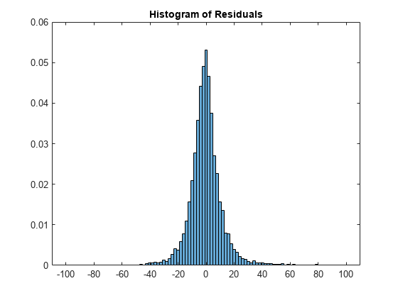
Assess and Adjust Model
Looking at the output p-values in the display, some variables might be unnecessary in the model. You can reduce the complexity of the model by removing these variables.
Examine the significance of the variables in the model more closely using anova.
a = anova(model)
a=9×5 table
                    SumSq        DF        MeanSq         F         pValue
                  __________    _____    __________    _______    __________

    Year               26.88        1         26.88    0.17533       0.67543
    Month             175.84        1        175.84     1.1469       0.28421
    DayofMonth         114.6        1         114.6    0.74749       0.38729
    DayOfWeek         3691.4        6        615.23     4.0129    0.00050851
    DepTime           705.42        1        705.42     4.6012      0.031964
    ArrDelay      1.2112e+07        1    1.2112e+07      79004             0
    Distance          8920.9        1        8920.9     58.188    2.5106e-14
    Hr                1047.5        1        1047.5     6.8321     0.0089613
    Error         2.5531e+06    16653        153.31
Based on the p-values, the variables Year, Month, and DayOfMonth are not significant to this model, so you can remove them without negatively affecting the model quality.
To explore these model parameters further, use interactive visualizations such as plotSlice, plotInterations, and plotEffects. For example, use plotEffects to examine the estimated effect that each predictor variable has on the departure delay.
plotEffects(model)
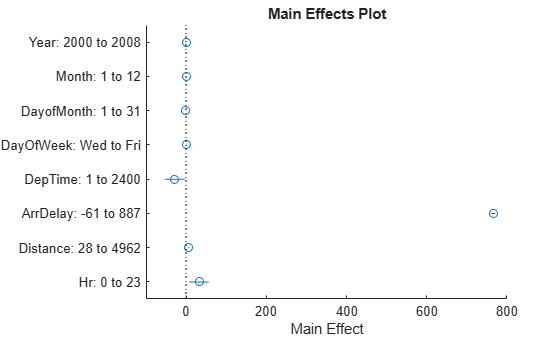
Based on these calculations, ArrDelay is the main effect in the model (it is highly correlated to DepDelay). The other effects are observable, but have much less impact. In addition, Hr was determined from DepTime, so only one of these variables is necessary to the model.
Reduce the number of variables to exclude all date components, and then fit a new model.
model2 = fitlm(dataTrain,'DepDelay ~ DepTime + ArrDelay + Distance')Evaluating tall expression using the Local MATLAB Session: - Pass 1 of 1: Completed in 0.46 sec Evaluation completed in 0.52 sec
model2 =
Compact linear regression model:
    DepDelay ~ 1 + DepTime + ArrDelay + Distance

Estimated Coefficients:
                   Estimate         SE         tStat       pValue
                   _________    __________    _______    __________

    (Intercept)      -1.4646       0.31696    -4.6207    3.8538e-06
    DepTime        0.0025087    0.00020401     12.297    1.3333e-34
    ArrDelay         0.80767     0.0028712      281.3             0
    Distance       0.0012981    0.00016886     7.6875    1.5838e-14


Number of observations: 16667, Error degrees of freedom: 16663
Root Mean Squared Error: 12.4
R-squared: 0.833,  Adjusted R-Squared: 0.833
F-statistic vs. constant model: 2.77e+04, p-value = 0
Model Development
Even with the model simplified, it can be useful to further adjust the relationships between the variables and include specific interactions. To experiment further, repeat this workflow with smaller tall arrays. For performance while tuning the model, you can consider working with a small extraction of in-memory data before scaling up to the entire tall array.
In this example, you can use functionality like stepwise regression, which is suited for iterative, in-memory model development. After tuning the model, you can scale up to use tall arrays.
Gather a subset of the data into the workspace and use stepwiselm to iteratively develop the model in memory.
subset = gather(dataTest);
Evaluating tall expression using the Local MATLAB Session:
- Pass 1 of 1: Completed in 0.27 sec
Evaluation completed in 0.28 sec
sModel = stepwiselm(subset,'ResponseVar','DepDelay')
1. Adding ArrDelay, FStat = 42200.3016, pValue = 0
2. Adding DepTime, FStat = 51.7918, pValue = 6.70647e-13
3. Adding DepTime:ArrDelay, FStat = 42.4982, pValue = 7.48624e-11
4. Adding Distance, FStat = 15.4303, pValue = 8.62963e-05
5. Adding ArrDelay:Distance, FStat = 231.9012, pValue = 1.135326e-51
6. Adding DayOfWeek, FStat = 3.4704, pValue = 0.0019917
7. Adding DayOfWeek:ArrDelay, FStat = 26.334, pValue = 3.16911e-31
8. Adding DayOfWeek:DepTime, FStat = 2.1732, pValue = 0.042528
sModel =
Linear regression model:
    DepDelay ~ 1 + DayOfWeek*DepTime + DayOfWeek*ArrDelay + DepTime*ArrDelay + ArrDelay*Distance

Estimated Coefficients:
                                Estimate          SE         tStat        pValue
                               ___________    __________    ________    __________

    (Intercept)                     1.1799        1.0675      1.1053       0.26904
    DayOfWeek_Mon                  -2.1377        1.4298     -1.4951       0.13493
    DayOfWeek_Tues                 -4.2868        1.4683     -2.9196     0.0035137
    DayOfWeek_Wed                  -1.6233         1.476     -1.0998       0.27145
    DayOfWeek_Thu                 -0.74772        1.5226    -0.49109       0.62338
    DayOfWeek_Fri                  -1.7618        1.5079     -1.1683        0.2427
    DayOfWeek_Sat                  -2.1121        1.5214     -1.3882       0.16511
    DepTime                     7.5229e-05    0.00073613     0.10219        0.9186
    ArrDelay                        0.8671      0.013836      62.669             0
    Distance                     0.0015163    0.00023426      6.4728    1.0167e-10
    DayOfWeek_Mon:DepTime        0.0017633     0.0010106      1.7448      0.081056
    DayOfWeek_Tues:DepTime       0.0032578     0.0010331      3.1534     0.0016194
    DayOfWeek_Wed:DepTime       0.00097506      0.001044     0.93398       0.35034
    DayOfWeek_Thu:DepTime        0.0012517     0.0010694      1.1705       0.24184
    DayOfWeek_Fri:DepTime        0.0026464     0.0010711      2.4707      0.013504
    DayOfWeek_Sat:DepTime        0.0021477     0.0010646      2.0174      0.043689
    DayOfWeek_Mon:ArrDelay        -0.11023      0.014744     -7.4767     8.399e-14
    DayOfWeek_Tues:ArrDelay       -0.14589      0.014814     -9.8482    9.2943e-23
    DayOfWeek_Wed:ArrDelay       -0.041878      0.012849     -3.2593     0.0011215
    DayOfWeek_Thu:ArrDelay       -0.096741      0.013308     -7.2693    3.9414e-13
    DayOfWeek_Fri:ArrDelay       -0.077713      0.015462     -5.0259    5.1147e-07
    DayOfWeek_Sat:ArrDelay        -0.13669      0.014652      -9.329    1.3471e-20
    DepTime:ArrDelay            6.4148e-05    7.7372e-06      8.2909    1.3002e-16
    ArrDelay:Distance          -0.00010512    7.3888e-06     -14.227    2.1138e-45


Number of observations: 8333, Error degrees of freedom: 8309
Root Mean Squared Error: 12
R-squared: 0.845,  Adjusted R-Squared: 0.845
F-statistic vs. constant model: 1.97e+03, p-value = 0
The model that results from the stepwise fit includes interaction terms.
Now try to fit a model for the tall data by using fitlm with the formula returned by stepwiselm.
model3 = fitlm(dataTrain,sModel.Formula)
Evaluating tall expression using the Local MATLAB Session:
- Pass 1 of 1: Completed in 0.47 sec
Evaluation completed in 0.51 sec
model3 =
Compact linear regression model:
    DepDelay ~ 1 + DayOfWeek*DepTime + DayOfWeek*ArrDelay + DepTime*ArrDelay + ArrDelay*Distance

Estimated Coefficients:
                                Estimate          SE         tStat        pValue
                               ___________    __________    ________    __________

    (Intercept)                   -0.31595       0.74499     -0.4241        0.6715
    DayOfWeek_Mon                 -0.64218        1.0473    -0.61316       0.53978
    DayOfWeek_Tues                -0.90163        1.0383    -0.86836       0.38521
    DayOfWeek_Wed                  -1.0798        1.0417     -1.0365       0.29997
    DayOfWeek_Thu                  -3.2765        1.0379      -3.157     0.0015967
    DayOfWeek_Fri                  0.44193        1.0813     0.40869       0.68277
    DayOfWeek_Sat                   1.1428        1.0777      1.0604       0.28899
    DepTime                      0.0014188    0.00051612      2.7489     0.0059853
    ArrDelay                       0.72526      0.011907      60.913             0
    Distance                     0.0014824    0.00017027      8.7059    3.4423e-18
    DayOfWeek_Mon:DepTime       0.00040994    0.00073548     0.55738       0.57728
    DayOfWeek_Tues:DepTime      0.00051826    0.00073645     0.70373       0.48161
    DayOfWeek_Wed:DepTime       0.00058426    0.00073695     0.79281        0.4279
    DayOfWeek_Thu:DepTime        0.0026229    0.00073649      3.5614    0.00036991
    DayOfWeek_Fri:DepTime        0.0002959    0.00077194     0.38332       0.70149
    DayOfWeek_Sat:DepTime      -0.00060921    0.00075776    -0.80396       0.42143
    DayOfWeek_Mon:ArrDelay       -0.034886      0.010435     -3.3432    0.00082993
    DayOfWeek_Tues:ArrDelay     -0.0073661      0.010113    -0.72837        0.4664
    DayOfWeek_Wed:ArrDelay       -0.028158     0.0099004     -2.8441     0.0044594
    DayOfWeek_Thu:ArrDelay       -0.061065      0.010381     -5.8821    4.1275e-09
    DayOfWeek_Fri:ArrDelay        0.052437      0.010927      4.7987    1.6111e-06
    DayOfWeek_Sat:ArrDelay        0.014205       0.01039      1.3671        0.1716
    DepTime:ArrDelay            7.2632e-05    5.3946e-06      13.464     4.196e-41
    ArrDelay:Distance          -2.4743e-05    4.6508e-06     -5.3203    1.0496e-07


Number of observations: 16667, Error degrees of freedom: 16643
Root Mean Squared Error: 12.3
R-squared: 0.837,  Adjusted R-Squared: 0.836
F-statistic vs. constant model: 3.7e+03, p-value = 0
You can repeat this process to continue to adjust the linear model. However, in this case, you should explore different types of regression that might be more appropriate for this data. For example, if you do not want to include the arrival delay, then this type of linear model is no longer appropriate. See Logistic Regression with Tall Arrays for more information.
Scale to Spark
A key capability of tall arrays in MATLAB and Statistics and Machine Learning Toolbox is the connectivity to platforms such as Hadoop and Spark. You can even compile the code and run it on Spark using MATLAB Compiler™. See Extend Tall Arrays with Other Products for more information about using these products:
Database Toolbox™
Parallel Computing Toolbox™
MATLAB® Parallel Server™
MATLAB Compiler™