Perform Incremental Learning and Track Performance Metrics Using Update Metrics Block
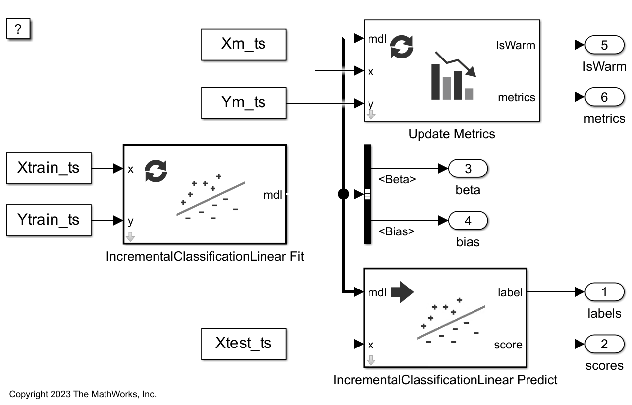
This example shows how to use the IncrementalClassificationLinear Fit, IncrementalClassificationLinear Predict, and Update Metrics blocks to perform incremental learning and track performance metrics in Simulink®. The IncrementalClassificationLinear Fit block fits a chunk of observations (predictor data) using a configured incremental linear model for binary classification (incrementalClassificationLinear) and outputs updated incremental learning model parameters as a bus signal. The IncrementalClassificationLinear Predict block accepts an IncrementalClassificationLinear model and a chunk of predictor data, and outputs the predicted labels for the observations. The Update Metrics block predicts labels for a chunk of predictor data using the incremental learning model, and outputs performance metrics.
Load and Preprocess Data
Load the human activity data set. Randomly shuffle the data.
load humanactivity
ndata = numel(actid);
rng(0,"twister") % For reproducibility
idx = randsample(ndata,ndata);
X = feat(idx,:);
Y = actid(idx);
For details on the data set, enter Description at the command line.
Responses can be one of five classes: Sitting, Standing, Walking, Running, or Dancing. Dichotomize the response by identifying whether the subject is moving (actid > 2).
Y = Y > 2;
Select 10,000 observations as the training set, and select 10,000 observations to track the model performance metrics.
n = 10000;
Xtrain = X(1:n,:);
Ytrain = Y(1:n,:);
Xmetrics = X(n+1:2*n,:);
Ymetrics = Y(n+1:2*n,:);
Create Incremental Learner Model
Create an incremental linear model for binary classification. Specify that the data has 60 predictors and that the data type of the responses is logical. Also specify to standardize the data using an estimation period of 500 observations before the Update Metrics block outputs performance metrics. Create a workspace variable linearMdl to store the initial incremental learning model.
Mdl = incrementalClassificationLinear(ClassNames=[false,true], ...
    NumPredictors=60,Standardize=true,EstimationPeriod=500, ...
    MetricsWarmupPeriod=500);
linearMdl = Mdl;
Create Input Data for Simulink
Simulate streaming data by dividing the training data into chunks of 50 observations. For each chunk, select a single observation as a test set to import into the IncrementalClassificationLinear Predict block.
numObsPerChunk = 50;
nchunk = floor(n/numObsPerChunk);
for j = 1:nchunk
    ibegin = min(n,numObsPerChunk*(j-1) + 1);
    iend = min(n,numObsPerChunk*j);
    idx = ibegin:iend;
    Xin(:,:,j) = Xtrain(idx,:);
    Yin(:,j) = Ytrain(idx);
    Xm_in(:,:,j) = Xmetrics(idx,:);
    Ym_in(:,j) = Ymetrics(idx);
    Xtest(1,:,j) = Xtrain(idx(1),:);
 end
Convert the training, metrics, and test set chunks into time series objects.
t = 0:size(Xin,3)-1;
Xtrain_ts = timeseries(Xin,t,InterpretSingleRowDataAs3D=true);
Ytrain_ts = timeseries(Yin',t,InterpretSingleRowDataAs3D=true);
Xm_ts = timeseries(Xm_in,t,InterpretSingleRowDataAs3D=true);
Ym_ts = timeseries(Ym_in',t,InterpretSingleRowDataAs3D=true);
Xtest_ts = timeseries(Xtest,t,InterpretSingleRowDataAs3D=true);
Open Provided Simulink Model
This example provides the Simulink model slexUpdateMetricsExample.slx, which includes the IncrementalClassificationLinear Fit, IncrementalClassificationLinear Predict, and Update Metrics blocks. The Simulink model is configured to use linearMdl as the initial model for incremental learning and classification.
Open the Simulink model slexUpdateMetricsExample.slx.
slName = "slexUpdateMetricsExample";
open_system(slName);
Simulate Model
Simulate the Simulink model to perform incremental learning, predict responses for the test set observations, and compute performance metrics. Export the simulation outputs to the workspace. You can use the Simulation Data Inspector (Simulink) to view the logged data of an Outport block.
simOut = sim(slName,"StopTime",num2str(numel(t)-1));
% Extract labels
yfit_sig = simOut.yout.getElement(1);
yfit_sl = squeeze(yfit_sig.Values.Data);

% Extract score values
scores_sig = simOut.yout.getElement(2);
scores_sl = squeeze(scores_sig.Values.Data);

% Extract beta values
beta_sig = simOut.yout.getElement(3);
beta_sl = squeeze(beta_sig.Values.Data);

% Extract bias values
bias_sig = simOut.yout.getElement(4);
bias_sl = squeeze(bias_sig.Values.Data);

% Extract IsWarm values
IsWarm_sig = simOut.yout.getElement(5);
IsWarm_sl = squeeze(IsWarm_sig.Values.Data);

% Extract metrics values
metrics_sig = simOut.yout.getElement(6);
metrics_sl = squeeze(metrics_sig.Values.Data);
At each iteration, the IncrementalClassificationLinear Fit block trains the model and updates the model parameters. The IncrementalClassificationLinear Predict block calculates the predicted label for the test set observation, and the Update Metrics block calculates the performance metrics.
Analyze Model During Training
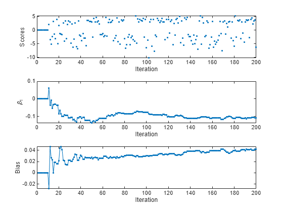
To see how the model parameters and scores evolve during training, plot them on separate tiles.
figure
tiledlayout(3,1);
nexttile
plot(scores_sl(1,:),".")
ylabel("Scores")
xlabel("Iteration")
xlim([0 nchunk])
nexttile
plot(beta_sl(1,:),".-")
ylabel("\beta_1")
xlabel("Iteration")
xlim([0 nchunk])
nexttile
plot(bias_sl,".-")
ylabel("Bias")
xlabel("Iteration")
xlim([0 nchunk])

During the estimation period, the IncrementalClassificationLinear Fit block estimates hyperparameters but does not fit the initial model (see incrementalRegressionLinear). Therefore, the score output of the IncrementalClassificationLinear Predict block, model beta coefficients, and model bias all equal 0 during the first 10 iterations. At the end of the estimation period, the IncrementalClassificationLinear Fit block updates the model parameters and predicts labels. The score values vary between approximately –10 and 5. The first beta coefficient drops significantly during the first 30 iterations following the estimation period, and then varies between –0.14 and –0.07 thereafter. The bias (intercept) term fluctuates initially and then gradually approaches 0.04.
Plot the IsWarm status indicator value and cumulative performance metric on separate tiles.
figure
tiledlayout(2,1);
nexttile
plot(IsWarm_sl,".")
ylabel("IsWarm")
xlabel("Iteration")
xlim([0 nchunk])
nexttile
plot(metrics_sl(:,1),".")
ylabel("Cumulative Metric (classiferror)")
xlabel("Iteration")
xlim([0 nchunk])
ylim([0 0.005])

After the estimation period, the Update Metrics block fits observations during the metrics warm-up period but does not calculate performance metrics. After the metrics warm-up period, IsWarm = 1 and the block calculates the performance metrics. In the provided Simulink model, the model performance metric is classiferror (the classification error). The cumulative classification error is –1 during the first 21 iterations, 0 for the next 23 iterations, and then varies between 0.001 and 0.003.
See Also
IncrementalClassificationLinear Fit | IncrementalClassificationLinear Predict | IncrementalRegressionLinear Fit | IncrementalRegressionLinear Predict | Update
Metrics | incrementalRegressionLinear | fit | predict | updateMetricsAndFit | updateMetrics