Analytical Model of Cantilever Truss Structure for Simscape

Define Model Parameters

The goal of this example is to analytically relate the displacement d to the uniform cross-section area parameter A for a particular bar in the cantilever truss structure. The governing equation is represented by $$M\frac{d^{2}x}{d{t}^2}+Kx=F$$. Here, d results from a load at the upper-right joint of the cantilever. The truss is attached to the wall at the leftmost joints.

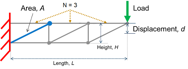
The truss bars are made of a linear elastic material with uniform density. The cross-section area A of the bar highlighted in blue (see figure) can vary. All other parameters, including the uniform cross-section areas of the other bars, are fixed. Obtain the displacement of the tip by using small and linear displacement assumptions.

First, define the fixed parameters of the truss.

Specify the length and height of the truss and the number of top horizontal truss bars.

L = 1.5;
H = 0.25;
N = 3;

Specify the density and modulus of elasticity of the truss bar material.

rhoval = 1e2;
Eval = 1e7;

Specify the cross-section area of other truss bars.

AFixed = 1;

Next, define the local stiffness matrix of the specific truss element.

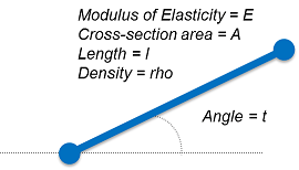
Compute the local stiffness matrix k and express it as a symbolic function. The forces and displacements of the truss element are related through the local stiffness matrix. Each node of the truss element has two degrees of freedom, horizontal and vertical displacement. The displacement of each truss element is a column matrix that corresponds to [x_node1,y_node1,x_node2,y_node2]. The resulting stiffness matrix is a 4-by-4 matrix.

syms A E l t real
G = [cos(t) sin(t) 0 0; 0 0 cos(t) sin(t)];
kk = A*E/l*[1 -1;-1 1];
k = simplify(G'*kk*G);
localStiffnessFn = symfun(k,[t,l,E])

localStiffnessFn(t, l, E) = 
$$\begin{array}{l}\left(\begin{array}{cccc}{\sigma }_2& {\sigma }_1& -{\sigma }_2& -{\sigma }_1\\ {\sigma }_1& {\sigma }_3& -{\sigma }_1& -{\sigma }_3\\ -{\sigma }_2& -{\sigma }_1& {\sigma }_2& {\sigma }_1\\ -{\sigma }_1& -{\sigma }_3& {\sigma }_1& {\sigma }_3\end{array}\right)\\ \\ \mathrm{where}\\ \\ \mathrm{ }{\sigma }_1=\frac{A\hspace{0.17em}\text{E}\hspace{0.17em}\sin \left(2\hspace{0.17em}t\right)}{2\hspace{0.17em}l}\\ \\ \mathrm{ }{\sigma }_2=\frac{A\hspace{0.17em}\text{E}\hspace{0.17em}{\cos \left(t\right)}^2}{l}\\ \\ \mathrm{ }{\sigma }_3=\frac{A\hspace{0.17em}\text{E}\hspace{0.17em}{\sin \left(t\right)}^2}{l}\end{array}$$

Compute the mass matrix in a similar way.

syms rho
mm = A*rho*l/6*[2 1;1 2];
m = simplify(G'*mm*G);
localMassFn = symfun(m,[t,l,rho]);

Now, define the bars of truss as a matrix bars. The indices for the bars, starting joints, and end joints are shown in the following figure.

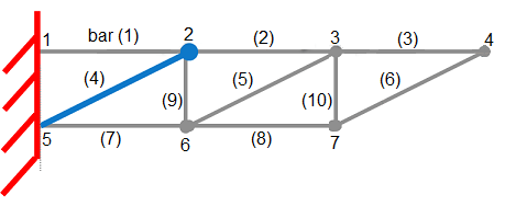
The number of rows of the matrix bars is the number of bars of the truss. The columns of bars have four elements, which represent the following parameters:

bars = zeros(2*N+2*(N-1),4);

Define the upper and diagonal bars. Note that the bar of interest is the (N+1)th bar or bar number 4 which is the first diagonal bar from the left.

for n = 1:N
    lelem = L/N;
    bars(n,:) = [lelem,0,n,n+1];
    lelem = sqrt((L/N)^2+H^2);
    bars(N+n,:) = [lelem,atan2(H,L/N),N+1+n,n+1];
end

Define the lower and vertical bars.

for n = 1:N-1
    lelem = L/N;
    bars(2*N+n,:) = [lelem,0,N+1+n,N+1+n+1];
    lelem = H;
    bars(2*N+N-1+n,:) = [lelem,pi/2,N+1+n+1,n+1];
end

Assemble Bars into Symbolic Global Matrices

The truss structure has seven nodes. Each node has two degrees of freedom (horizontal and vertical displacements). The total number of degrees of freedom in this system is 14.

numDofs = 2*2*(N+1)-2

numDofs = 
14

The system mass matrix M and system stiffness matrix K are symbolic matrices. Assemble local element matrices from each bar into the corresponding global matrix.

K = sym(zeros(numDofs,numDofs));
M = sym(zeros(numDofs,numDofs));
for j = 1:size(bars,1)
    % Construct stiffness and mass matrices for bar j.
    lelem = bars(j,1); telem = bars(j,2);
    kelem = localStiffnessFn(telem,lelem,Eval);
    melem = localMassFn(telem,lelem,rhoval);
    n1 = bars(j,3); n2 = bars(j,4);
    % For bars that are not within the parameterized area A, set the stiffness
    % and mass matrices to numeric values. Note that although the values
    % kelem and melem do not have symbolic parameters, they are still
    % symbolic objects (symbolic numbers).
    if j ~= N+1
        kelem = subs(kelem,A,AFixed);
        melem = subs(melem,A,AFixed);
    end
    % Arrange the indices.
    ix = [n1*2-1,n1*2,n2*2-1,n2*2];
    % Embed local elements in system global matrices.
    K(ix,ix) = K(ix,ix) + kelem;
    M(ix,ix) = M(ix,ix) + melem;
end

Eliminate degrees of freedom attached to the wall.

wallDofs = [1,2,2*(N+1)+1,2*(N+1)+2]; % DoFs to eliminate
K(wallDofs,:) = [];
K(:,wallDofs) = [];
M(wallDofs,:) = [];
M(:,wallDofs) = [];

F is the load vector with a load specified in the negative Y direction at the upper rightmost joint.

F = zeros(size(K,1),1);
F(2*N) = -1;

To extract the Y displacement at the upper rightmost joint, create a selection vector.

c = zeros(1,size(K,1));
c(2*N) = 1;

Create Simscape Equations from Exact Symbolic Solution for Static Case

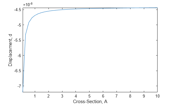
Find and plot the analytical solution for the displacement d as a function of A. Here, K\F represents the displacements at all joints and c selects the particular displacements. First, show the symbolic solution representing numeric values using 16 digits for compactness.

d_Static = simplify(c*(K\F));
vpa(d_Static,16)

ans = 
$$-\frac{0.00000001118033988749895\hspace{0.17em}\left(504.7737197247586\hspace{0.17em}{A}^2+384.7213595499958\hspace{0.17em}A+22.3606797749979\right)}{A\hspace{0.17em}\left(1.28\hspace{0.17em}A+0.8944271909999158\right)}$$

fplot(d_Static,[AFixed/10,10*AFixed]);
hold on;
xlabel('Cross-Section, A');
ylabel('Displacement, d');
title('')

Convert the result to a Simscape equation ssEq to use inside a Simscape block. To display the resulting Simscape equation, remove the semicolon.

syms d
ssEq = simscapeEquation(d,d_Static);

Display the first 120 characters of the expression for ssEq.

strcat(ssEq(1:120),'...')

ans = 
'd == (sqrt(5.0)*(A*2.2e+2+A*cos(9.272952180016122e-1)*2.0e+2+sqrt(5.0)*A^2*1.16e+2+sqrt(5.0)*1.0e+1+A^2*cos(9.2729521800...'

Compare Numeric and Symbolic Static Solutions

Compare the exact analytical solution and numeric solution over a range of A parameter values. The values form a sequence from AFixed to 5*AFixed in increments of 1.

AParamValues = AFixed*(1:5)';
d_NumericArray = zeros(size(AParamValues));
for k=1:numel(AParamValues)
    beginDim = (k-1)*size(K,1)+1;
    endDim = k*size(K,1);
    % Create a numeric stiffness matrix and extract the numeric solution.
    KNumeric = double(subs(K,A,AParamValues(k)));
    d_NumericArray(k) = c*(KNumeric\F);
end

Compute the symbolic values over AParamValues. To do so, call the subs function, and then convert the result to double-precision numbers using double.

d_SymArray = double(subs(d_Static,A,AParamValues));

Visualize the data in a table.

T = table(AParamValues,d_SymArray,d_NumericArray)

T=5×3 table
    AParamValues    d_SymArray     d_NumericArray
    ____________    ___________    ______________

         1          -4.6885e-06     -4.6885e-06  
         2          -4.5488e-06     -4.5488e-06  
         3          -4.5022e-06     -4.5022e-06  
         4          -4.4789e-06     -4.4789e-06  
         5          -4.4649e-06     -4.4649e-06  

Approximate Parametric Symbolic Solution for Frequency Response

A parametric representation for the frequency response H(s,A) can be efficient for quickly examining the effects of parameter A without resorting to potentially expensive numeric calculations for each new value of A. However, finding an exact closed-form solution for a large system with additional parameters is often impossible. Therefore, you typically approximate a solution for such systems. This example approximates the parametric frequency response near the zero frequency as follows:

Use vpa to speed up calculations.

digits(32);
K = vpa(K);
M = vpa(M);

Compute the LU decomposition of K.

[LK,UK] = lu(K);

Create helper variables and functions.

iK = @(x) UK\(LK\x);
iK_M = @(x) -iK(M*x);
momentPre = iK(F);

Define a frequency series corresponding to the first three moments. Here, s is the frequency.

syms s
sPowers = [1 s^2 s^4];

Set the first moment, which is the same as d_Static in the previous computation.

moments = d_Static;

Compute the remaining moments.

for p=2:numel(sPowers)
    momentPre = iK_M(momentPre);
    for pp=1:numel(momentPre)
        momentPre(pp) = taylor(momentPre(pp),A,AFixed,'Order',3);
    end
    moment = c*momentPre;
    moments = [moments;moment];
end

Combine the moment terms to create the approximate analytical frequency response Happrox.

HApprox = sPowers*moments;

Display the first three moments. Because the expressions are large, you can display them only partially.

momentString = arrayfun(@char,moments,'UniformOutput',false);
freqString = arrayfun(@char,sPowers.','UniformOutput',false);
table(freqString,momentString,'VariableNames',{'FreqPowers','Moments'})

ans=3×2 table
    FreqPowers                                                                                                                                                                                                           Moments                                                                                                                                                                                                       
    __________    _____________________________________________________________________________________________________________________________________________________________________________________________________________________________________________________________________________________________________________________________________________________________________________________________________________________

     {'1'  }      {'-(5^(1/2)*(220*A + 200*A*cos(8352332796509007/9007199254740992) + 116*5^(1/2)*A^2 + 10*5^(1/2) + 40*A^2*cos(8352332796509007/9007199254740992) + 40*A^2 + 20*5^(1/2)*A + 152*5^(1/2)*A^2*cos(8352332796509007/9007199254740992) + 36*5^(1/2)*A^2*cos(8352332796509007/4503599627370496)))/(200000000*A*(A - A*cos(8352332796509007/4503599627370496) - 5^(1/2)*cos(8352332796509007/9007199254740992) + 5^(1/2)))'}
     {'s^2'}      {'0.000000000084654421099019119162064316556812*(A - 1)^2 - 0.000000000079001242991597407593795324876303*A + 0.0000000004452470882909076005654298481594'                                                                                                                                                                                                                                                             }
     {'s^4'}      {'0.000000000000012982169746567833536274593916742*A - 0.000000000000015007141035503798552656353179406*(A - 1)^2 - 0.000000000000045855285883001825767717087472451'                                                                                                                                                                                                                                                  }

Convert the frequency response to a MATLAB function containing numeric values for A and s. You can use the resulting MATLAB function without Symbolic Math Toolbox.

HApproxFun = matlabFunction(HApprox,'vars',[A,s]);

Compare Purely Numeric and Symbolically Derived Frequency Responses

Vary the frequency from 0 to 1 in logspace, and then convert the range to radians.

freq = 2*pi*logspace(0,1);

Compute the numeric values of the frequency response for A = AFixed*perturbFactor, that is, for a small perturbation around A.

perturbFactor = 1 + 0.25;
KFixed = double(subs(K,A,AFixed*perturbFactor));
MFixed = double(subs(M,A,AFixed*perturbFactor));
H_Numeric = zeros(size(freq));
for k=1:numel(freq)
    sVal = 1i*freq(k);
    H_Numeric(k) = c*((sVal^2*MFixed + KFixed)\F);
end

Compute the symbolic values of the frequency response over the frequency range and A = perturbFactor*AFixed.

H_Symbolic = HApproxFun(AFixed*perturbFactor,freq*1i);

Plot the results.

figure
loglog(freq/(2*pi),abs(H_Symbolic),freq/(2*pi),abs(H_Numeric),'k*');
xlabel('Frequency');
ylabel('Frequency Response');
legend('Symbolic','Numeric');

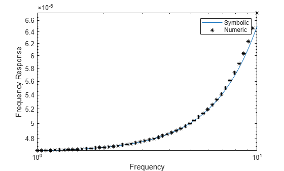
The analytical and numeric curves are close in the chosen interval, but, in general, the curves diverge for frequencies outside the neighborhood of s = 0. Also, for values of A far from AFixed, the Taylor approximation introduces larger errors.