Explore Single-Period Asset Arbitrage
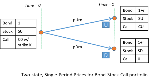
This example explores basic arbitrage concepts in a single-period, two-state asset portfolio. The portfolio consists of a bond, a long stock, and a long call option on the stock.
It uses these Symbolic Math Toolbox™ functions:
equationsToMatrixto convert a linear system of equations to a matrix.linsolveto solve the system.Symbolic equivalents of standard MATLAB® functions, such as
diag.
This example symbolically derives the risk-neutral probabilities and call price for a single-period, two-state scenario.
Define Parameters of the Portfolio
Create the symbolic variable r representing the risk-free rate over the period. Set the assumption that r is a positive value.
syms r positive
Define the parameters for the beginning of a single period, time = 0. Here S0 is the stock price, and C0 is the call option price with strike, K.
syms S0 C0 K positive
Now, define the parameters for the end of a period, time = 1. Label the two possible states at the end of the period as U (the stock price over this period goes up) and D (the stock price over this period goes down). Thus, SU and SD are the stock prices at states U and D, and CU is the value of the call at state U. Note that .
syms SU SD CU positive
The bond price at time = 0 is 1. Note that this example ignores friction costs.
Collect the prices at time = 0 into a column vector.
prices = [1 S0 C0]'
prices =
Collect the payoffs of the portfolio at time = 1 into the payoff matrix. The columns of payoff correspond to payoffs for states D and U. The rows correspond to payoffs for bond, stock, and call. The payoff for the bond is 1 + r. The payoff for the call in state D is zero since it is not exercised (because ).
payoff = [(1 + r), (1 + r); SD, SU; 0, CU]
payoff =
CU is worth SU - K in state U. Substitute this value in payoff.
payoff = subs(payoff, CU, SU - K)
payoff =
Solve for Risk-Neutral Probabilities
Define the probabilities of reaching states U and D.
syms pU pD real
Under no-arbitrage, eqns == 0 must always hold true with positive pU and pD.
eqns = payoff*[pD; pU] - prices
eqns =
Transform equations to use risk-neutral probabilities.
syms pDrn pUrn real;
eqns = subs(eqns, [pD; pU], [pDrn; pUrn]/(1 + r))
eqns =
The unknown variables are pDrn, pUrn, and C0. Transform the linear system to a matrix form using these unknown variables.
[A, b] = equationsToMatrix(eqns, [pDrn, pUrn, C0]')
A =
b =
Using linsolve, find the solution for the risk-neutral probabilities and call price.
x = linsolve(A, b)
x =
Verify the Solution
Verify that under risk-neutral probabilities, x(1:2), the expected rate of return for the portfolio, E_return equals the risk-free rate, r.
E_return = diag(prices)\(payoff - [prices,prices])*x(1:2);
E_return = simplify(subs(E_return, C0, x(3)))
E_return =
Test for No-Arbitrage Violations
As an example of testing no-arbitrage violations, use the following values: r = 5%, S0 = 100, and K = 100. For SU < 105, the no-arbitrage condition is violated because pDrn = xSol(1) is negative (SU >= SD). Further, for any call price other than xSol(3), there is arbitrage.
xSol = simplify(subs(x, [r,S0,K], [0.05,100,100]))
xSol =
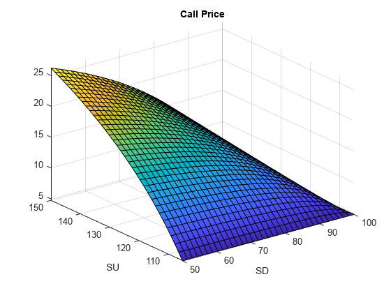
Plot Call Price as a Surface
Plot the call price, C0 = xSol(3), for 50 <= SD <= 100 and 105 <= SU <= 150. Note that the call is worth more when the "variance" of the underlying stock price is higher for example, SD = 50, SU = 150.
fsurf(xSol(3), [50,100,105,150])
xlabel SD
ylabel SU
title 'Call Price'
Reference
Advanced Derivatives, Pricing and Risk Management: Theory, Tools and Programming Applications by Albanese, C., Campolieti, G.