lambertw
Lambert W function
Syntax
Description
Examples
The Lambert W function W(x) is a set of
solutions of the equation x =
W(x)eW(x).
Solve this equation. The solution is the Lambert W function.
syms x W
eqn = x == W*exp(W);
solve(eqn,W)
ans =
lambertw(0, x)
Verify that branches of the Lambert W function are valid solutions of the
equation x = W*eW:
k = -2:2;
eqn = subs(eqn,W,lambertw(k,x));
isAlways(eqn)
ans =
  1×5 logical array
1 1 1 1 1Depending on its arguments, lambertw can
return floating-point or exact symbolic results.
Compute the Lambert W functions for these numbers. Because the numbers are not symbolic objects, you get floating-point results.
A = [0 -1/exp(1); pi i];
lambertw(A)
ans =
   0.0000 + 0.0000i  -1.0000 + 0.0000i
   1.0737 + 0.0000i   0.3747 + 0.5764i
lambertw(-1,A)
ans =
     -Inf + 0.0000i  -1.0000 + 0.0000i
  -0.3910 - 4.6281i  -1.0896 - 2.7664i
Compute the Lambert W functions for the numbers converted to symbolic objects.
For most symbolic (exact) numbers, lambertw returns unresolved
symbolic calls.
A = [0 -1/exp(sym(1)); pi i];
W0 = lambertw(A)
W0 =
[               0,             -1]
[ lambertw(0, pi), lambertw(0, 1i)]
Wmin1 = lambertw(-1,A)
Wmin1 =
[             -Inf,              -1]
[ lambertw(-1, pi), lambertw(-1, 1i)]
Convert symbolic results to double by using double.
double(W0)
ans =
   0.0000 + 0.0000i  -1.0000 + 0.0000i
   1.0737 + 0.0000i   0.3747 + 0.5764i
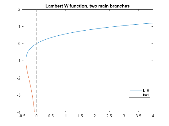
Plot the two main branches, and , of the Lambert W function.
syms x
fplot(lambertw(x))
hold on
fplot(lambertw(-1,x))
hold off
axis([-0.5 4 -4 2])
title('Lambert W function, two main branches')
legend('k=0','k=1','Location','best')

Plot the principal branch of the Lambert W function on the complex plane.
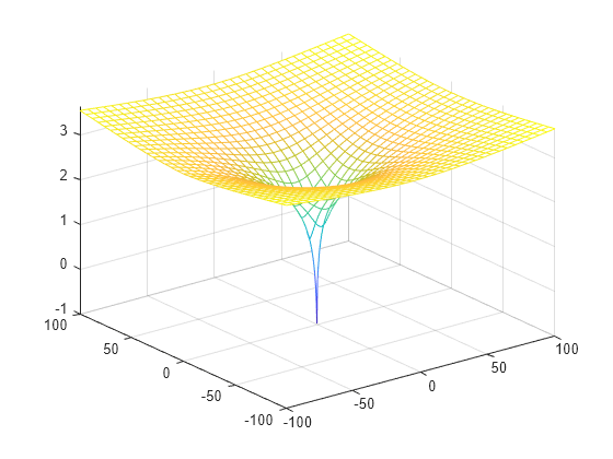
Plot the real value of the Lambert W function by using fmesh. Simultaneously plot the contours by setting 'ShowContours' to 'On'.
syms x y
f = lambertw(x + 1i*y);
interval = [-100 100 -100 100];
fmesh(real(f),interval,'ShowContours','On')

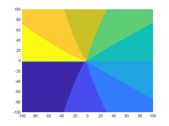
Plot the imaginary value of the Lambert W function. The plot has a branch cut along the negative real axis. Plot the contours separately.
fmesh(imag(f),interval)

fcontour(imag(f),interval,'Fill','on')

Plot the absolute value of the Lambert W function.
fmesh(abs(f),interval,'ShowContours','On')

Input Arguments
Input, specified as a number, vector, matrix, or array, or a symbolic number, variable, array, function, or expression.
At least one input argument must be a scalar, or both arguments must be vectors
or matrices of the same size. If one input argument is a scalar and the other is a
vector or matrix, lambertw expands the scalar into a vector or
matrix of the same size as the other argument with all elements equal to that
scalar.
Branch of Lambert W function, specified as an integer, a vector or matrix of integers, a symbolic integer, or a symbolic vector or matrix of integers.
At least one input argument must be a scalar, or both arguments must be vectors
or matrices of the same size. If one input argument is a scalar and the other is a
vector or matrix, lambertw expands the scalar into a vector or
matrix of the same size as the other argument with all elements equal to that
scalar.
More About
The Lambert W function W(x) represents the solutions y of the equation for any complex number x.
For complex x, the equation has an infinite number of solutions y = lambertW(k,x) where k ranges over all integers.
For all real x ≥ 0, the equation has exactly one real solution y = lambertW(x) = lambertW(0,x).
For real x where , the equation has exactly two real solutions. The larger solution is represented by y = lambertW(x) and the smaller solution by y = lambertW(–1,x).
For , the equation has exactly one real solution y = –1 = lambertW(0, –exp(–1)) = lambertW(–1, -exp(–1)).
References
[1] Corless, R.M., G.H. Gonnet, D.E.G. Hare, D.J. Jeffrey, and D.E. Knuth. "On the Lambert W Function." Advances in Computational Mathematics, Vol. 5, pp. 329–359, 1996.
Version History
Introduced before R2006a
MATLAB Command
You clicked a link that corresponds to this MATLAB command:
Run the command by entering it in the MATLAB Command Window. Web browsers do not support MATLAB commands.
选择网站
选择网站以获取翻译的可用内容,以及查看当地活动和优惠。根据您的位置,我们建议您选择:。
您也可以从以下列表中选择网站:
如何获得最佳网站性能
选择中国网站(中文或英文)以获得最佳网站性能。其他 MathWorks 国家/地区网站并未针对您所在位置的访问进行优化。
美洲
- América Latina (Español)
- Canada (English)
- United States (English)
欧洲
- Belgium (English)
- Denmark (English)
- Deutschland (Deutsch)
- España (Español)
- Finland (English)
- France (Français)
- Ireland (English)
- Italia (Italiano)
- Luxembourg (English)
- Netherlands (English)
- Norway (English)
- Österreich (Deutsch)
- Portugal (English)
- Sweden (English)
- Switzerland
- United Kingdom (English)