Validate Simulink Model Using Symbolic Math Toolbox

Open Live Script

This example shows how to model a bouncing ball, which is a classical hybrid dynamic system. This model includes both continuous dynamics and discrete transitions. It uses the Symbolic Math Toolbox™ to help explain some of the theory behind ODE solving in the Simulation of Bouncing Ball (Simulink).

Assumptions

The ball rebounds with no angle
There is no drag
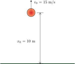
Height at time t=0 is 10 m
Thrown with upwards velocity of 15 m/s

Derivation

The coefficient of restitution is defined as

$C_{r} = v_{b} - v_{a} / u_{a} - u_{b}$

where v is the speed of object before impact and u is the speed after.

We split the second order differential equation

$\frac{d^{2} h}{d t^{2}} = - g$

into

$\frac{d h}{d t} = v$ discretized as $\frac{h (t + Δ t) - h (t)}{Δ t} = v (t)$

and

$\frac{d v}{d t} = - g$ discretized as $\frac{v (t + Δ t) - v (t)}{Δ t} = - g$

We will use basic 1st order numerical integration using forward Euler.

$h (t + Δ t) = h (t) + v (t) Δ t$

$v (t + Δ t) = v (t) - g Δ t$

Solve the Problem Analytically

Using the Symbolic Math Toolbox, we can approach the problem analytically. This allows us to solve certain problems more easily, such as determining precisely when the ball first hits the ground (below).

Declare our symbolic variables.

syms g t H(t) h_0 v_0

Split the second order differential equation $\frac{d^{2} h}{d t^{2}} = - g$ into $\frac{d h}{d t} = v$ and $\frac{d v}{d t} = - g$ .

Dh = diff(H);
D2h = diff(H, 2) == g

D2h(t) = 
 $\frac{\partial^{2}}{\partial t^{2}} H (t) = g$

Solve the ODE using dsolve:

eqn = dsolve(D2h, H(0) == h_0, Dh(0) == v_0)

eqn = 
 $\frac{g t^{2}}{2} + v_{0} t + h_{0}$

Parametrically explore the parabolic profile of motion using subs:

eqn = subs(eqn, [h_0, v_0, g], [10, 15, -9.81])

eqn = 
 $- \frac{981 t^{2}}{200} + 15 t + 10$

Find the time at which the ball hits the ground by solving for zero:

assume(t > 0)
tHit = solve(eqn == 0)

tHit = 
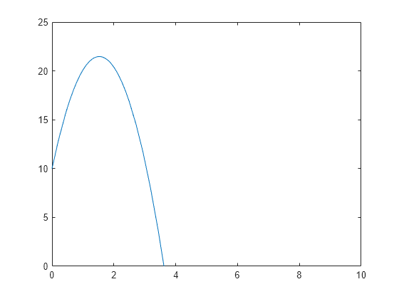
 $\frac{20 \sqrt{5} \sqrt{26}}{109} + \frac{500}{327}$

Visualize the solution:

fplot(eqn,[0 10])
ylim([0 25])

Figure contains an axes object. The axes object contains an object of type functionline.

Format your exact results using variable precision arithmetic with vpa:

disp(['The ball with an initial height of 10m and velocity of 15m/s will hit the ground at ' char(vpa(tHit, 4)) ' seconds.'])

The ball with an initial height of 10m and velocity of 15m/s will hit the ground at 3.621 seconds.

Solve the Problem Numerically

Setup Simulation Parameters

Properties of the ball

c_bounce = .9;        % Bouncing's coefficient of restitution; perfect restitution would be 1

Properties of the simulation

gravity  = 9.8;       % Gravity's acceleration (m/s)
height_0 = 10;        % Initial height at time t=0 (m)
velocity_0=15;        % Initial velocity at time t=0 (m/s)

Declaring the simulation time step

dt = 0.05;            % Animation timestep (s)
t_final = 25;         % Simulate period (s)
t = 0:dt:t_final;     % Timespan
N = length(t);        % Number of iterations

Initialize simulation quantities

h=[];                 % Height of the ball as a function of time (m)
v=[];                 % Velocity of the ball (m/sec) as a function of time (m/s)
h(1)=height_0;
v(1)=velocity_0;

Simulate the bouncing ball (we will use basic 1st order numerical integration using forward Euler):

for i=1:N-1
       
    v(i+1)=v(i)-gravity*dt;
    h(i+1)=h(i)+v(i)*dt;
    
    % When the ball bounces (the height is less than 0), 
    % reverse the velocity and recalculate the position.
    % Using the coefficient of restitution
    if h(i+1) < 0
        
       v(i)=-v(i)*c_bounce;
       v(i+1)=v(i)-gravity*dt;
       h(i+1)=0+v(i)*dt;

    end
    
end

Visualize and validate the simulation

plot(t,h,'o')
hold on 
fplot(eqn,[0 10])
title('Height over time')
ylim([0 25])
hold off

Figure contains an axes object. The axes object with title Height over time contains 2 objects of type line, functionline. One or more of the lines displays its values using only markers

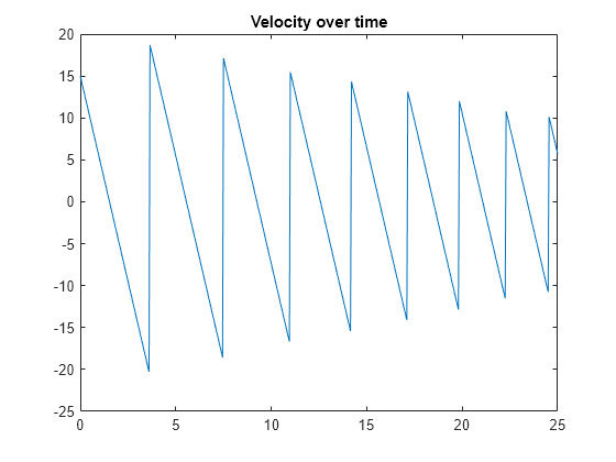
plot(t,v)
title('Velocity over time')

Figure contains an axes object. The axes object with title Velocity over time contains an object of type line.

Validate Numerics with Analytics

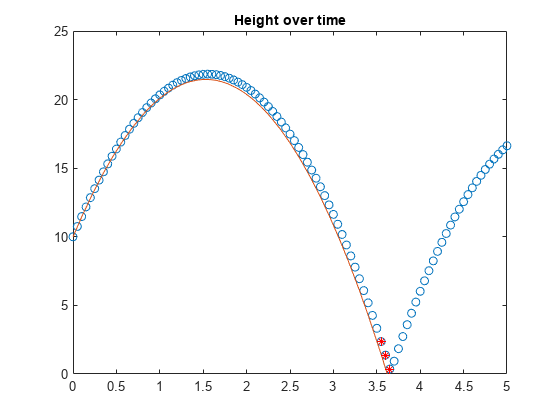
Compare your analytical results with your numeric results.

As a reminder the time of impact was:

disp(['The ball with an initial height of 10m and velocity of 15m/s will hit the ground at ' char(vpa(tHit, 4)) ' seconds.'])

The ball with an initial height of 10m and velocity of 15m/s will hit the ground at 3.621 seconds.

From the numerical simulation we can find the closest value in the simulation when $h (t_{i}) \approx 0$

i = ceil(double(tHit/dt));
t([i-1 i i+1])

ans = 1×3

    3.5500    3.6000    3.6500

plot(t,h,'o')
hold on 
fplot(eqn,[0 10])
plot(t([i-1 i i+1 ]),h([i-1 i i+1 ]),'*R')
title('Height over time')
xlim([0 5])
ylim([0 25])
hold off

Figure contains an axes object. The axes object with title Height over time contains 3 objects of type line, functionline. One or more of the lines displays its values using only markers